
Manage storage by building software RAID with the Linux mdadm command.
Linux Software RAID
Redundant array of inexpensive disks (RAID) allows you to combine multiple physical storage devices (solid-state and hard drives) into one or more logical units, or virtual storage devices. The reasons to create these virtual storage devices can include data redundancy, availability, or performance, or to achieve all goals. The number of the RAID level describes the combination of reliability, availability, performance, and capacity. For example, RAID 0 stripes data across multiple storage devices to improve performance, whereas RAID 1 mirrors data across storage devices to improve data availability and resiliency. Other RAID levels and combinations of RAID levels are possible, as well.
The original paper on RAID defined what are termed the standard RAID levels still in use. For a better understanding, I discuss them briefly in the following sections then present the Linux software RAID mdadm command, a powerful tool for building Linux storage servers.
RAID 0
This RAID level focuses on performance by striping across two or more storage devices, with no effort to achieve data redundancy; therefore, if a storage device that is part of the RAID 0 group is lost, you will likely lose data. However, RAID 0 gives the best performance for a set of storage devices and uses all of the capacity of the devices for storing user data. Figure 1 (GFDL license) illustrates a two-device RAID 0 group. For the sake of discussion, although the image looks like two spinning disks and not solid-state devices (SSDs), the principle is the same.
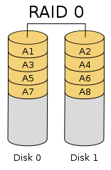 Figure 1: RAID 0 layout (from Cburnett at Wikipedia under the GFDL license).
In the case of writing to the RAID group, the first block of data is written to A1, which happens to be on the first device on the left. The next block of data is written to A2 on the second storage device on the right. The third block is written to A3, and so on, in a round robin fashion. This is referred to as striping data across the two devices. As the I/O rate goes up, the data is written to two blocks virtually at the same time, so you get two times the performance of a single device.
Reading data also benefits from the data block layout. A read starts with the block where the data is located on either device. With two devices, the next block, usually on the next device, can be read at the same time. Again, this effectively doubles the read performance of the RAID group compared with a single device.
RAID 0 is fantastic on performance and storage utilization. The RAID group uses all the space on both storage devices and performance improves almost by a factor of the number of devices (e.g., times two for two storage devices). With Linux software RAID, you can have as many storage devices in your RAID 0 group as you want. However, if you lose a storage device in the group and you can’t completely recover the device, you will lose data. If you are using RAID 0 and can’t afford to lose data, be sure to make a backup.
RAID 1
RAID 1 performs data mirroring, completely focusing on data availability, meaning a copy of the data that is written to one storage device is also written to one or more other storage devices. You can even use three or more storage devices for keeping copies of the data.
Figure 2 illustrates a two-device RAID 1 group. Notice how the device on the left is exactly the same as on that the right; that is, they are mirrors of each other.
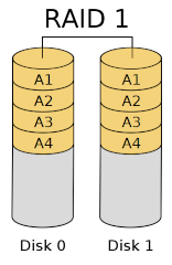 Figure 2: RAID 1 layout (from Cburnett at Wikipedia under the GFDL license).
As previously mentioned, when data is written to the RAID 1 group, it is written to each storage device. RAID 1 has very poor storage utilization, because even if you have N storage devices, you only have the capacity of one storage device. Write performance is also limited to the performance of a single storage device. However, read performance can be very good because any of the devices can be used to retrieve the data.
Finally, data availability is very good. You can lose all but one storage device and not lose any data. Note that this is not a backup solution, but a data availability approach to data storage.
RAID 2-4
These RAID levels, although defined in the original RAID paper, are really not used any more except in certain very specific cases, so I won’t cover them here.
RAID 5
This RAID level distributes data across storage devices in a group and computes the parity data, which is also distributed across the storage devices. Parity is a simple form of error detection, wherein a data bit is added to a string of binary code. For a given binary string, a parity bit is computed and added to the string. If part of the data in the binary string is lost, from the remaining data and the parity bit, the missing data can be recomputed. For RAID 5, the parity data is computed and spread across the storage devices along with the data. If a storage device fails, the data can be recovered from the parity information.
A RAID 5 group requires at least three storage devices. If a storage device is lost and the group starts recovering the data from the parity and a second device is lost, then you will lose data, because only a single copy of the parity data is written to the group.
Figure 3 shows a four-device RAID 5 group. The data stripes are written as A, B, C, and D and are color coded. Any block with a p appended indicates a parity block that is part of a stripe.
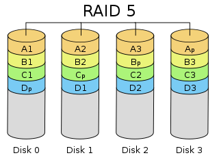 Figure 3: RAID 5 layout (from Cburnett at Wikipedia under the GFDL license).
Data is written to a stripe that lies across three of the devices, with the fourth storage device storing the parity bit of the data in the stripe. As an example, the data is written to the stripe A1, A2, A3. As this stripe is filled with data, the parity of the data is computed and written to Ap (the parity block).
When data is written to the B stripe, the parity is not put on the same device as the A stripe. The A stripe parity block is on the fourth storage device from the left. The B stripe puts the block on the third storage device from the left. The process continues for the C and D stripes that also use different storage devices than the preceding stripe for its parity block. In this way parity is distributed across the storage devices, decreasing the likelihood of losing data.
If you lose a storage device (e.g., Disk 2), you lose the A3, C2, and D2 blocks as well as the B stripe parity (block Bp). However, you can reconstruct A3 from the data in A1 and A2 along with the parity block Ap. The same is true for reconstructing C2 and D3 by using the remaining blocks and the parity blocks for that stripe.
Note that you haven’t lost any data in the B stripe. The data blocks B1, B2, and B3 are still there. But to make sure you don’t lose any data you need to recover the Bp block (the B strip parity block). To recover Bp, you recompute the parity from B1, B2, and B3.
A RAID 5 group lets you lose a single storage device and not lose data because either the data or the parity for the missing blocks on the lost device can be found on the remaining devices. Moreover, many RAID 5 groups will include a “hot spare” storage device. When a device in the RAID group fails and the reconstruction of missing data begins, the data blocks are written to the hot spare. If you don’t have a hot spare, then reconstruction cannot begin. If you don’t quickly put another storage device in the server, then if a second device fails, you will lose data.
The storage efficiency of RAID 5 is quite good. In a group of N storage devices, (N – 1) are storing data. Read performance is very good because more than one device can be used to read the data. Write performance is reasonable because you can write to (N – 1) devices as you would RAID 0 (e.g., write a stripe of data).
RAID 6
Somewhat similar to RAID 5, two copies of the parity are written to two storage devices in the RAID group. This method uses more space to store parity information, but it can survive the loss of two storage devices without losing data. Note that RAID 6 was not part of the original RAID definition but was later created to deal with the problem of a second storage device failure during a rebuild.
Figure 4 shows a RAID 6 group, which requires a minimum of four devices. The layout of the data and parity blocks is not unique as with RAID 5, wherein a parity block shifts one device over for the next stripe. RAID 6 data and parity blocks can be laid out in various ways, as long as the RAID group can continue to execute read and write operations to all of the virtual devices in the RAID group. However, you must be certain that a storage device is not dedicated to just storing parity data.
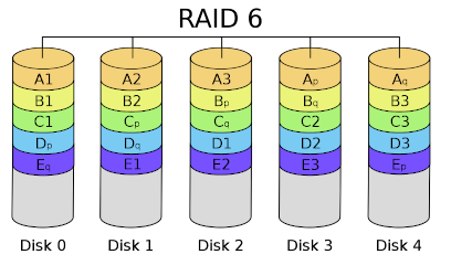 Figure 4: RAID 6 layout (from Cburnett at Wikipedia under the GFDL license).
RAID Level Characteristics
RAID levels have particular characteristics (Table 1; N is the number of storage devices in the RAID group):
- A space efficiency of 1 is the maximum (think of it as 100%).
- Fault Tolerance is the number of storage devices that can be lost without a loss of data.
- Read and write performance is relative to a single storage device in the RAID group.
Table 1: RAID Level Characteristics
| RAID Level | Minimum No. of Storage Devices | Space Efficiency | Fault Tolerance | Read Performance | Write Performance |
|---|---|---|---|---|---|
| 0 | 2 | 1 | None | N | N |
| 1 | 2 | 1/N | N – 1 storage device failures | N | 1 |
| 5 | 3 | 1 – (1/N) | One storage device failure | N | N – 1 (full stripe) |
| 6 | 4 | 1 – (2/N) | Two storage device failures | N | N – 2 (full stripe) |
The table presents some interesting information. You can think of the space efficiency as a percentage. For example, with four storage devices (N = 4), RAID 0 is 100% space efficient (it’s always 100% for RAID 0), RAID 1 is 1/4 = 0.25 (25%), RAID 5 is 0.8 (80%), and RAID 6 is 0.5 (50%).
From the table, you can also estimate the read and write performance of the various RAID levels. The table presents performance relative to the performance of a single storage device. With four storage devices, the read performance of RAID 0 is 4 (i.e., four times a single storage device), and the write performance is 4 (four times a single storage device). RAID 1 has a read performance of 4 (four times a single device), and the write performance is 1 (the performance of a single device). For RAID 5 the read performance is 4 and the write performance for a full stripe is 3. RAID 6 is slightly different with a read performance of 4 and a full stripe write performance of 2.
Nested RAID
Although not part of the original definition of RAID, “nested” RAID combinations can be created with the Linux software RAID tools. An example of a nested RAID level could be RAID 10. In this case, two RAID levels are “nested.”
To understand nested RAID, you start with the far-right number and proceed to the left. For RAID 10, this means the “top” level RAID is RAID 0. Underneath this read level are RAID 1 groups. To construct such a beastie, you take at least two partitions and create at least two RAID 1 groups with a total of four storage devices (partitions). Then you take these RAID 1 groups and create a RAID 0 group. This process creates the RAID 10 group, on top of which you create the filesystem.
Figure 5 shows a possible RAID 10 group of four devices. (Note that the Wikipedia article for Nested RAID levels uses the notation RAID 1+0.)
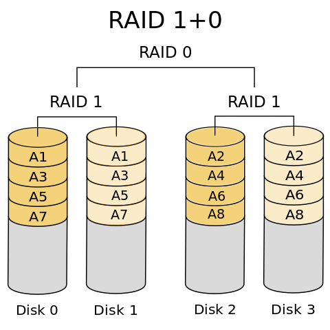 Figure 5: RAID 10 layout (from NudelSuppe at Wikipedia under the GFDL license).
Nested RAID allows you to combine the features of two RAID levels. RAID 10 gives great performance (twice the RAID 1 performance), but unlike RAID 0, you can lose a storage device and still not lose any data thanks to RAID 1 at the lower level. While read performance is very good, the write performance is not as good because of the RAID 1 at the lower level. However, the write performance is better than RAID 1 because of RAID 0 at the top level.
You can easily see why people are using something like RAID 50 or RAID 60 to add better performance and space efficiency at the lower level. Furthermore, nothing limits you to RAID levels. You can easily construct a RAID 100 (the famous “Triple Lindy”) or even a RAID 500 or RAID 600 with Linux software RAID.
mdadm Software RAID Tool
The fundamental tool used for Linux software RAID is mdadm. Online literature discusses how to use mdadm to create various RAID levels, so I won’t go over the commands to create all of the RAID levels; however, but I will cover RAID 0, RAID 1, and RAID 5.
Creating a RAID 0 Group
To begin, assume that you have four storage devices, and you want to create a RAID 0 group. For the sake of discussion, create a single partition on each of the devices. To create the RAID 0 group, enter:
# mdadm --verbose --create /dev/md0 --level=0 \
  --raid-devices=4 /dev/sdc1 /dev/sdd1 /dev/sde1 /dev/sdf1
This command creates a multiple device (md) within Linux. Sys admins often use md at the beginning of the device name to indicated that it is a multiple device, but you can name it anything you want (e.g., /dev/alt_wesley_crusher_die_die_die – if you know, you know). In this case, the device is /dev/md0. After creating the RAID 0 group, you can create a filesystem on it with /dev/md0 as the device.
The other options in the command are pretty self-explanatory. I like to use --verbose in case of a problem. Plus, when I’m ready to deploy software RAID in production, I redirect the output to a file to document everything.
Creating a RAID 1 Group
The mdadm command to create the RAID 1 md is:
# mdadm --verbose --create /dev/md0 --level=1 \
  --raid-devices=2 /dev/sdc1 /dev/sdd1
Remember that RAID 1 is theh mirroring of two storage devices.
Creating a RAID 5 Group
Building a RAID 5 group with mdadm is very similar:
# mdadm --verbose --create /dev/md0 --level=5 \
  --raid-devices=3 /dev/sdc1 /dev/sdd1 /dev/sde1
Recall that you need to use at least three storage devices in a RAID 5 group.
Useful Information
A number of tools and techniques can help you manage and monitor software RAID. The command
cat /proc/mdstat
gives you some really useful information, such as the “personality” of the RAID (i.e., the RAID level) and the status of the devices in the RAID group. This last item is very useful because it reveals whether the RAID group is degraded (i.e., you lost a device) and the status of device recovery if you are rebuilding data or resyncing the storage devices.
In the past I have used this command in conjunction with watch for active monitoring of the status of the RAID array, especially when recovering from a storage device failure.
The main mdadm software RAID command has some useful options to get information about the status and configuration of the RAID array. For example,
mdadm –detail
gives you some great output. Adding the --scan option scans the RAID arrays to give you some basic information.
You can also use the mdadm command with a specific md device to get lots of information about the array. For example
mdadm --detail /dev/md0
outputs details about the array, including the RAID level, total number of devices, and the number of devices in the RAID group. It also gives you the status of the RAID group, the chunk size (which is important if you are concerned about performance), and information about the state of the individual storage devices in the group.
You can use the mdadm command to manage the RAID group (e.g., stopping the group, marking a device as “failed,”removing a device from the group, or adding a spare storage device to the group). I recommend reading the mdadm man page if you are going to use software RAID.
RAID Built In to the Filesystem
You can build any filesystem you want on top of a multiple device; however, some filesystems have RAID built in. The two that come to mind immediately are ZFS (OpenZFS) and Btrfs. I won’t cover these filesystems or using RAID with them here. If you are interested, a bit of searching will find a great deal. However, be sure to read the most recent articles because features and commands may have changed.
Software RAID Summary
With the advent of many CPU cores and lots of memory, it is very easy to use Linux software RAID to achieve great performance. You can use the logical volume manager (LVM) and software RAID together to create a very useful storage solution. The details of creating the solution are not the subject of this article, so if you want to build your own storage solution, please spend some time reading as much as you can and be sure to experiment and test before putting anything into production. Also, thoroughly document everything.
I’m sure someone will send a nastygram to me if I don’t include this last comment: RAID is not a backup solution. RAID is all about data performance and data accessibility and availability; for data reliability, you need a real backup solution for that. You have been warned.
Summary
The Linux software RAID mdadm tool covers all the standard RAID levels that were described in the first RAID paper. RAID 6 was added down the road to address the issue of the fragility of RAID 5 when a storage device fails. The same tool allows you to create whatever RAID level you want.
You can also use mdadm to create nested RAID levels – one RAID level on top of another. Two-digit nested RAID levels such as RAID 10 can be created by first creating RAID 1 groups and then combining with RAID 0 on top. Nothing could stop you from creating three nested RAID levels (e.g., RAID 100), but just like the Triple Lindy, the degree of difficulty increases dramatically.
I’m still moving along the path of answering the question of how to manage storage. Answering that question by illustrating how to build Linux storage servers will get you to the point of discussing tools to manage the users either on Linux or a proprietary filesystem.