Fast and Lean

Preparing the Data

As discussed, each active file access has a cursor in its opened file that describes its current position in the file. Libiotrace does not directly trace the current cursor position, also known as the offset, but you can find the function calls that alter the offset, along with additional information about the number of bytes the cursor is changed in the database. These details allow the determination of the current cursor offset before and after each function call.

A Python script [6] performs this task. With the influxdb_client Python library, the script loads time series libiotrace data from the InfluxDB instance. For easier handling, the script transforms the data into a pandas.DataFrame [7] and adjusts its structure.

In the next step, it processes the time-sorted data for each file access. Each function has different additional data traced by libiotrace that describes how the offset changes. With this information – and according to the function used – the script calculates the offset after each call and adds the value to a new column of the dataframe. The influxdb_client library writes the enriched data, in the form of a dataframe, to the InfluxDB instance for further use.

First Insights

A dashboard in Grafana enables an explorative visualization of the previously enriched InfluxDB data created by libiotrace . Both the tool's preparatory work and the finished solution involve the use of a Grafana dashboard to gain insights.

In the pre-work dashboard, interactive pie charts let you navigate from top to bottom, exploring the traced processes, function calls, and files used by the traced program. In the drill-down view shown in Figure 6, you can click on the pie charts to view more detailed information, progressing from left to right. This approach makes the libiotrace data accessible, allowing you to gain insights.

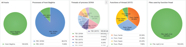Figure 6: Pie chart panels of a Grafana dashboard showing the data from an InfluxDB time series database.

A connected pre-work time series diagram shows how the offset of file accesses on the selected file (Figure 7) and the cursor position of each file access changes over time. Each color stands for a distinct file access ID.

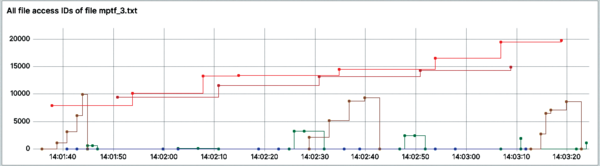Figure 7: The course of the offsets of all file accesses on a selected file, distinguished by color.

Selecting a specific file access ID lets you see the cursor position's course in detail, with the called functions made visible (Figure 8). This method highlights when a function is repeated consecutively.

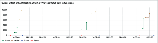Figure 8: The detailed offset course of the yellow file accesses in Figure 7. The colors represent the called functions.

The ability to show function calls of other file accesses alongside the selected file access allows for a quick comparison of sequential calls. As you can see in Figure 9, the vertical lines display the timestamps of relevant functions of other file accesses on the same file and directly indicates when such a call occurs between two consecutive function calls of the same type by the selected file access.

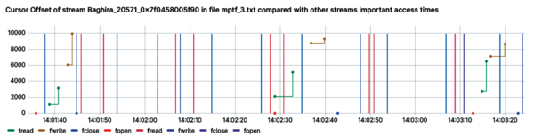Figure 9: This chart is similar to Figure 7 but has all other relevant function calls of other file accesses displayed as vertical lines.

An additional challenge arises during rapid function calls in a program. Libiotrace measures the timestamps with a very high level of detail to ensure consistency. Although InfluxDB can also handle this level of detail, Grafana only supports timestamps up to milliseconds in its dashboards.

For multiple points with timestamps differing only at the microsecond level or deeper, Grafana shows them as a single point in the time series diagrams, which results in missing data in the visualizations. More importantly, it prevents a visual sequential comparison.

The script tackles this issue because the sequence of the function calls is the most important property when looking for optimizations. When data points have different timestamps on a more detailed level, but the timestamps would be truncated to the same timestamp because of Grafana's granularity, the later timestamp is adjusted to the next millisecond.

Additionally, the script accounts for consecutive calls and adjusts their position when necessary to maintain the correct sequence. Grafana then recognizes both data points as different points and visualizes them as such. The script makes this small adjustment to the real timestamps to achieve the dashboard's goal of displaying the sequence of file accesses and their function calls.

This first step in identifying problematic situations where unnecessary frequent and small function calls occur has limitations, including the explorative nature of the dashboard, which makes the optimization process quite time consuming. Also, this visualization only covers the simple sequential comparison of file accesses and does not allow a detailed comparison at the offset level.

Instead of manually analyzing such cases with the dashboard, the goal was to automate the detection of these optimizations and visualize them in a clear and explanatory way. The tool explained in this article performs this automated optimization discovery.

Implementation Details

After the script processes the data created by libiotrace to include information about the current offset, the tool then uses this information to identify optimization opportunities. It does so by iterating over all file accesses and filtering the entire dataframe to include only the data of the current file access.

Each row in this dataframe contains information such as the timestamp, function name, offset after the call, and accessed file name, among other details. The script then iterates through the filtered dataframe row by row in chronological order, searching for consecutive occurrences of a function. A dictionary collects all rows involved in function calls that are being called more than once consecutively and bundles them in lists.

The next step iterates over the collected information inside the dictionary. For each function call bundle, the script takes the timestamps of the first and the last call. It uses these timestamps to filter the original dataframe of all file accesses on the current file. This retrieves all function calls from other file accesses that took place between the repeated function calls. This filtered dataframe contains all the information about what happened inside the file between the first and last bundled repeated function calls, allowing the script to work with a reduced dataframe.

The script then checks whether each repeated function pair within the bundle can be optimized. To do so, it uses the data in the reduced dataframe to retrieve all function calls on the file from other file accesses during the time between the consecutive function calls.

With this information, the script classifies each pair into self-defined optimization categories.

• Category 0 means it cannot be optimized.
• Category 1 means it can easily be optimized.
• Category 2 means that although one or more other intermediate calls exist, optimization is still possible.
• Category 3 means bail out, because the file access function is not handled.

For each consecutive repeated function call pair, the script creates a new optimization point, regardless of the classification, and adds it to a dataframe containing all analyzed possible optimizations.

An optimization point contains all shared information by both calls, as well as the timestamps of each call and the classified category of the optimization with additional information on the classification reasons. Because this data still is time series data and will be written into the InfluxDB instance to visualize it in Grafana, each point has a timestamp set to the mean of the consecutive functions' timestamps. In this way, you can directly see in a time series diagram to which function calls an optimization point belongs.

To classify each possible optimization and add additional information, the script runs each pair through several checks.