
Your parallel application is running fine, but you want it to run faster. Naturally, you use more and more cores, and everything is great; however, suddenly performance starts decreasing. What just happened?
Why Isn’t Your Application Scaling?
Your application is running in parallel across multiple cores and multiple nodes, and you are overjoyed, as you should be. You are seeing parallel processing in action, and for some HPC enthusiasts, this is truly thrilling. At this point, you want the application to run faster, so you try using more cores (processes). You expect that as the number of processes increases, the wall clock time should decrease. A faster running application is, of course, one of the goals of parallel processing. However, as you steadily increase the number of processes, something goes terribly wrong – the wall clock time actually starts increasing.
You have just found the scalability limit of the application – that is, the point at which the wall clock time stops decreasing. Any number of processes greater than the scalability limit results in increasing wall clock time. Many times people will ask why this happens. Answering this question will increase your knowledge of HPC and your application, so I’ll look at one of the fundamental reasons for scalability limitations.
Introducing Gene Amdahl
Underlying the scalability limit is something called Amdahl’s Law, proposed by Gene Amdahl in 1967. (As a side note, Gene Amdahl was the first person to use FUD in its current meaning.) Figure 1 describes Amdahl’s Law.
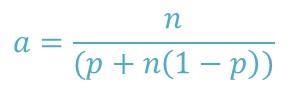 Figure 1: Amdahl’s law.
In this equation, a is the application speedup, n is the number of processors, and p is the parallel fraction, or the fraction of the application that is parallelizable (0 to 1).
In an absolutely perfect world, the parallelizable fraction of the application is 1 (p = 1), or perfectly parallelizable. In this case, Amdahl’s Law reduces to a = n. That is, the speedup is linear with the number of cores and is also infinitely scalable. You can keep adding processors, and the application will get faster.
At the opposite end, if the parallelizable code fraction is zero (p = 0), then Amdahl’s Law reduces to a = 1, which means that no matter how many cores or processes are used, performance does not improve (wall clock time does not change).
To better understand how Amdahl’s Law works, consider a theoretical application that is 80% parallelizable (20% serial). For one process, the wall clock time is assumed to be 1,000 seconds. This means that 200 seconds of the wall clock time is the serial portion of the application. Also, vary the number of processes from 1 to 64. Figure 2 plots the resulting wall clock time on the y-axis versus the number of processes.
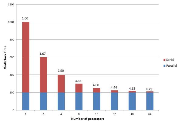 Figure 2: Example application and the influence of Amdahl’s Law.
In Figure 2, the blue portion of each bar is the serial wall clock time, and the red portion is the wall clock time of the parallel portion of the application. Above each bar is the speedup, a, based on the number of processes. Notice that with one process, the sum of the serial portion and the parallel portion, is 1,000 seconds, with the serial portion being 200 seconds and the parallel portion 800 seconds. Amdahl’s Law says the speedup is 1.00 (i.e., the starting point).
Notice that as the number of processes increase, the wall clock time of the parallel portion decreases. The speed-up increases from 1.00 with 1 process to 4.71 with 64 processes. However, also notice that the wall clock time for the serial portion of the application does not change. It stays at 200 seconds regardless of the number of processes.
Figure 2 can explain a great deal about how parallel applications scale. The most important thing to notice is that total wall clock time will never be faster than the serial time. Because the parallelization fraction is greater than 0 but less than 1, the speedup, a, reaches some limit as n, the number of processors, goes to infinity. In the case of this theoretical application, the speedup limit is 5.0. With a little math and a little computation, the asymptotic value of a is as shown in Figure 3.
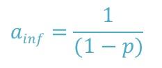 Figure 3: Asymptote of Amdahl’s Law.
For my theoretical application with p = 0.8, this works out to 5, just as the computations indicated. For p = 1, or perfectly scalable, a goes to infinity as n goes to infinity, which also matches the earlier observations. For p = 0, or no parallelizable fraction, a stays at 1, which also matches the previous observation.
On the basis of the plot in Figure 2, you can make the observation that, fundamentally, the scalability of the application is limited by serial time. This observation bothers some people when talking about a parallel, and not a serial, application. How far you can scale your parallel application is driven by the serial portion of your application.
Further examination of Figure 2 illustrates a property of Amdahl’s Law: The application is infinitely scalable if p > 0. The wall clock time will continue to shrink as you increase the number of processes. As the number of processes gets large, the wall clock time reduction is extremely small, but it is non-zero. However, recall that applications have been observed to have a scaling limit, after which the wall clock time increases. Why does Amdahl’s Law say that the applications can continue to reduce wall clock time?
The difference between Amdahl’s Law and real-life is that Amdahl’s Law assumes an infinitely fast network. That is, data can be transferred infinitely fast from one process to another (zero latency and infinite bandwidth). In real life, this isn’t true. All networks have non-zero latency and limited bandwidth, so data is not communicated infinitely fast but in some finite amount of time.
Another way to view Amdahl’s law is as a guide to where you should concentrate your resources to improve performance. I’m going to assume you have done everything you can to improve the parallel portion of the code. You are using asynchronous data transfers, you limit the number of collective operations, you are using a very low latency and high bandwidth network, you have profiled your application to understand the MPI portion, and so on. At this point, Amdahl’s Law says that to get better performance, you need to focus on the serial portion of your application.
Whence Does Serial Come?
The parts of an application that contribute to the serial portion of the overall application really depend upon your application and algorithm. “Serial” performance has several sources, but usually the predominant is I/O. When the application starts, it will most likely need to read an input file so that all of the processes have the information. Some applications also need to write data at some point while it runs. At the end of the application, it will likely write its results.
Typically these I/O steps take place in a single process. One reason is to avoid collisions during I/O, particularly during writes. If two processes open the same file and try writing to it, and the filesystem can’t handle multiple writes, then there is the definite possibility that the data could be written incorrectly. For example, if process 1 is supposed to write data first, followed by process 2, what happens if process 2 actually writes first followed by process 1? The answer is: You get a mess. However, with careful programming, you can have multiple processes write to the same file, but you as the programmer have to be very careful that each process does not try to write where another process is writing. This can take a great deal of work.
Another reason for using a single process for I/O is that most of the time it’s easy. The first process in an MPI application is the “rank-0” process. When the application does any I/O, the rank-0 process alone does it. In the case of reads, it will read the input data and send it to the other processes (mpi_send/mpi_isend/mpi_bcast from the rank-0 process and mpi_recv/mpi_irecv/mpi_bcast for the non-rank-0 processes). For writes, it is the opposite: The non-rank-0 processes send their data to the rank-0 process, which does I/O on behalf of all processes.
Having a single MPI process take care of I/O on behalf of the other processes by exchanging data creates a serial bottleneck in an application because only one processes is doing I/O, forcing the other processes to wait. Plus, the network has a limited amount of bandwidth and finite latency, sometimes causing processes to wait. If you want your application to scale, you need to reduce the amount of serial work taking place in the application. You have a couple of ways to do this. The first, which I already mentioned, is to have each process do its own I/O. This approach requires careful coding, or you could accidentally corrupt the data files.
The most common way to have all the processes perform I/O is to use MPI-IO, which is an extension of MPI incorporated in MPI-2 that allows you to perform I/O from all of the MPI processes in an application (or a subset). It is beyond the scope of this article to discuss MPI-IO, but just remember it can be a tool to help you reduce the serial portion of your application by parallelizing the I/O.
Before you decide to modify your application to parallelize I/O, it is a really good idea to understand whether I/O is a significant portion of the total application run time. If the I/O portion of your application is fairly small (the definition of “fairly small” is up to you), then it might not be worth rewriting the I/O portion of the application. An earlier article I wrote discusses various ways to effect I/O profiling of your application.
If serial I/O is not a significant portion of your application, then you might need to look for other sources of serial performance. Tracking down these sources can be difficult and tedious, but it is usually worthwhile because it improves scalability and application performance – and who doesn’t like speed?
Summary
Writing a useful parallel application is a wonderful accomplishment, and you will want to improve its performance. However, you might notice that at a certain point, increasing the number of processors used in the application doesn’t necessarily decrease the wall clock time of execution.
The first explanation for this behavior is described by Amdahl’s Law. This law illustrates the theoretical speedup of an application when running with more processes and how it is limited by the serial performance of the application. At some point, your application will not run appreciable faster unless you have a very small serial portion.
One of the big sources of serial bottlenecks in an application is I/O. Although I didn’t spend much time discussing it, examining the amount of time an application spends on I/O is an important step in understanding the serial portion of your application. Several tools and libraries can help you parallelize the I/O portion of your application; however, at some fundamental level, the application has to read input files and write output, limiting the scalability of the application (the scalability limit).
The goal is to push this limit to the largest number of processes possible, so get out there and improve the serial portion of your applications!