
The Warewulf cluster is ready to run HPC applications. Now, it’s time to build a development environment.
Warewulf Cluster Manager – Part 3
In the first two Warewulf articles, I finished the configuration of Warewulf so that I could run applications and do some basic administration on the cluster. Although there are a plethora of MPI applications, many of them need to be built. Additionally, you might want to write your own. Both require a development environment of compilers, libraries, and MPI libraries and tools. In this article, I show how you can easily create a development environment for Warewulf clusters.
Introduction
HPC clusters are a very interesting topic in and of themselves. How do you easily create and deploy clusters? How do manage them? How do you monitor them? These are all interesting questions and, depending on your interests, really enjoyable topics, But at the heart of HPC clusters is the need to run or create applications, or both, parallel or serial. For running applications, you need compilers, libraries, and MPI (Message Passing Interface) libraries and tools. Although it seems like a simple concept – and for single systems it is – clusters require you to think differently.
Clusters are disparate in terms of the OS, so you have to pay attention to how they are deployed and what tool sets are on each node. One could argue that the development and run-time environment has nothing to do with the deployment tools, and indeed, in the case of this article, one could argue that Warewulf has nothing to do with a development and run-time environment for clusters. However, I disagree. Keeping track of what packages and applications are installed on each node is of paramount importance, and this means the cluster toolkit becomes an integral part of the approach. For clusters, I see two approaches for a development or run-time environment: (1) a brute force approach or (2) a smart approach. In this article, I present the second approach for creating a development and run-time environment building on the Warewulf articles up to this point.
The brute force way to deploy a development and run-time environment for parallel applications is fairly simple – just put everything on each node and call it a day. Although brute force seems fairly simple, in general, this approached might not be the best, going back to some of the fundamental arguments for stateless nodes. By putting the tools on each node, you have to pay very close attention to versioning, so the versions of all of the tools are the same on each node. If not, there is the potential for problems, and I have seen them before.
A much more elegant approach, one that I call “smart,” is to put as many of the tools as possible on an NFS filesystem or some other common filesystem and then only put the minimum necessary on the nodes. This greatly reduces the problem of version skew between nodes. Plus, you can further reduce version skew to a minimum if you use a stateless cluster tool so that a node is simply rebooted to get the correct versions of tools. This makes Warewulf a wonderful tool for a development and run-time environment.
In this article I’m going to illustrate with several examples how one might create and deploy a development and run-time environment. I’m going to use two MPI toolkits – MPICH2 and Open MPI – and a BLAS library, Atlas (Automatically Tuned Linear Algebra Software), as an example of a pure library that is used by applications. Initially, I will be using the default compilers that come with Scientific Linux 6.2 for compiling. Finally, just to complicate things a bit more, I’m going to install a second compiler that can be used for all of these toolkits and libraries. To tie it all together, I’m going to use Environment Modules to show how you can use multiple toolkits or any other packages in the development environment. The use of Environment Modules is extremely important and makes your life infinitely easier.
Recall that there are four articles in this series about deploying Warewulf in HPC Clusters. The first two articles covered the initial setup of Warewulf and rounding out Warewulf to get the system ready for running HPC applications. The fourth article will add a number of the classic cluster tools, such as Torque and Ganglia, that make clusters easier to operate and administer.
For this article as with the previous one, I will use the exact same system as in the first article, running Scientific Linux 6.2 (SL6.2). The purpose of this article is not to show you how to build various toolkits for the best performance or illustrate how to install packages on Linux. Rather, it is to use these toolkits as examples of how to build your HPC development and run-time environment with Warewulf. At the same time, I’m choosing to work with toolkits commonly used in HPC, so I’m not working with something obscure; rather, these toolkits have proven to be very useful in HPC (at least in my humble opinion). I’m also choosing to build the toolkits from source rather than install them from an RPM (where possible). This allows me to have control over where they are installed and how they are built.
Useful Preliminary Packages
Today’s processors are becoming more and more complex and, in many ways, more non-uniform. For example, the latest AMD processors have two integer cores sharing a large floating-point (FP) unit. Alternatively, one of the integer cores can use the entire FP unit. Intel now has the PCI-Express controller in the processor, so if you have multiple sockets you have to pay attention to which core has a process utilizing a network interface to minimize traffic between the sockets. Consequently, you have to pay attention to where you place processes within the system. For both processors, process placement can have a big effect on performance.
Two tools can help. The first is numactl (Non-Uniform Memory Access [NUMA] Controls). This tool allows you to start processes on certain physical hardware and control memory access for these processes. This is an extremely useful toolkit for today’s hardware, particularly in HPC, where we want to squeeze every last ounce from the hardware.
The second toolset, hwloc (HardWare Locality), is a very useful toolkit because it gives you the tools and interfaces to abstract all of the non-uniformity of modern systems such as those that I previously mentioned. I’ve found it to be an invaluable tool for understanding the hardware layout from the perspective of the OS. Open MPI can use hwloc for proper placement of MPI processes.
Fortunately, for SL6.2, these packages are already built as RPMs, so installing them on the master node is as easy as:
yum install numactl
and
yum install hwloc
Depending on how you built the master node originally, numactl might already be installed because it comes with many basic installations. If not, it’s easy to install.
One tool I really like in hwloc is called lstopo, which gives you a graphical view of your hardware layout as the hwloc abstraction sees it. For example, for my generic hardware on the master node, the graphical output looks like Figure 1.
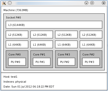 Figure 1: Example lstopo output
The graphical output shows you each socket (in this case, one), the cache structure (L3, L2, and L1), the cores (in this case, four), and the physical units (PUs) for each core (in this case, only 1 PU per core). It also shows you how the cores and the PUs are enumerated by the OS. That is, which core is number 0, which core is number 1, and so on. This can be very handy when you have complicated NUMA hardware.
Now that the tools are installed on the master node, it’s generally a good idea to install them in the VNFS (virtual node filesystem) that I’ve been using, which requires a little more attention to detail. If you recall in the second article, I was able to install individual packages into my VNFS on the master node. First, I’ll install numactl to illustrate how this is done. The output (Listing 1) has had some details removed to shorten it, as noted with the phrase [cut].
Notice that it also installs Perl, making the total size of the packages about 11MB, even though numactl itself is only 54KB. In the grand scheme of things, 11MB is not very much space, but if this amount of space is valuable, you have two choices: (1) don’t install numactl, or (2) build it yourself on the master node and use NFS to share it with the compute nodes.
The first option is up to you. My home system didn’t really need it because the physical layout is simple (see Figure 1), but for completeness sake, I think it’s important to install it. Again, it’s up to you.
The second option is also up to you. I have not built numactl by hand, so I don’t know the options or dependencies in doing so. But just be sure to build it so it installs in an NFS-exported filesystem from the master node (e.g., /opt).
I’m also going to install hwloc in the VNFS because it could prove very useful for tools such as Open MPI. To make my life easier, I’m going to follow the same installation procedure I used for numactl. The output (Listing 2) has also had some things removed to shorten it, as noted with the phrase [cut].
I think it’s always important to examine the output to understand the dependencies that come with the package. In this case, hwloc itself is 1.0MB, but the sum of it and all of the dependencies is 11MB. Again, this might or might not seem like a large amount to you. It’s your decision if you want to install it on the VNFS, install on an NFS filesystem from the master node, or not worry about it all. In my opinion, both numactl and hwloc are very important with today’s NUMA hardware. Therefore, I installed them in my VNFS. At this point, because I updated the VNFS, I should go back and rebuild it, but I’m going to wait because I want to get through the first round of development packages before I do that (no sense in doing it more times than needed).
MPI Libraries and Tools Using Default Compilers
MPI (Message Passing Interface) is the lingua franca for parallel computing today. Although you have other options for writing parallel code, a vast majority of today’s parallel code is being written with MPI. Consequently, it makes sense to have at least one, if not two, MPI toolkits on a cluster.
Several open source toolkits are available, but for the purposes of this article, I will stick to those that support Ethernet. In particular, I will focus on the ones that are commonly used: (1) MPICH2, and (2) Open MPI. In the following subsections, I’ll first build and install MPICH2 on the master node. Then, I’ll do the same for Open MPI. Finally, I’ll build and install a very common math library called BLAS using a tool called Atlas to generate the library.
For building and installing toolkits, I follow a set of practices that I put in place a while ago. If you like, you can think of them as standard processes, or habits even, but the intent is to save time and create something of a paper trail, so I can follow what I originally did. I will try to point out my practices, but you are not obligated to follow them by any means. However, I do highly recommend you develop some sort of standard practices so you too can create a paper trail.
The first practice I follow is where I put the toolkits when building them. By default I have the root user build and install the toolkits, and I do it in a subdirectory named src so that the full path looks like /root/src. I could have a user build the toolkits and then have root install them but I’ve found that it’s easier to just do everything as root. However, you need to be careful so you don’t inadvertently do something disastrous.
The second practice is to install the toolkits in a standard location. You have several possibilities, but I put all of mine in /opt on the master node. This is where I put “optional” packages that aren’t necessarily specific to the toolkit. Plus /opt is NFS-exported to the compute nodes, so I only need to do this once. Although you could install them on every compute node, that’s costly for a stateless cluster such as the Warewulf cluster I’ve been developing in this series. Instead, it’s just as easy to install the toolkits in a directory on the master node that is NFS-exported to the compute nodes.
I will discuss other practices I use when building and installing toolkits in the subsequent sections. Again, you don’t have to follow these practices, but it is important to develop some sort of standard practice. This will keep you from pulling out your hair and making a more supportable HPC cluster.
MPICH2 Using Default Compilers
If you’ve read the previous Warewulf article, you might know that a great number of Linux packages can be built from source with three simple steps:
- ./configure
- make
- make install
MPICH2 is no exception. As with much code, it is rather easy to build and install. One standard practice I follow is to examine the options included with configure, so I can chose which options I want to use. To do this, I typically just grab the output of ./configure using the script command:
% script configure.help
% ./configure --help
(output flashes on the screen)
^d
This dumps the output from the help option to a file named configure.help. Then, I can use the normal Linux tools, such as more or vi, to look at the help options and select the ones I want to use.
A third practice I have developed is that once I have the options I want, I create a quick script in the root directory of the toolkit so I know what options I used when building the toolkit. In the interest of standardization, I always name the file conf.jeff, so I can then go to a directory for a toolkit and look at conf.jeff to find what options I used in building the application. For MPICH2 on my system, the following shows what conf.jeff looks like:
./configure --prefix=/opt/mpich2-1.5b1 --enable-fc --enable-f77 --enable-romio --enable-mpe --with-pm=hydra
Notice that I install the toolkit into /opt/mpich2-1.5b1. I always install into a directory that reflects the version of the toolkit (making things easier for tracking the toolkit and version).
Once I have created conf.jeff, I change the permissions, using something like
chmod 700 conf.jeff
which allows me to execute it. Another standard practice I follow is to capture the output from the configuration in a file. To do this, I again use the script command, putting the output to a file before I execute the conf.jeff script:
% script conf.jeff.out
% ./conf.jeff
...
^d
This allows me to look back through the configuration output for anything that might be “weird.” Once I am satisfied, I then do the usual, make followed by make install. However, be sure to read the INSTALL file or README file that comes with each toolkit because some are different.
Once I have the toolkit configured, I’m ready to build it. I like to capture all of the standard output (stdout) when I build the toolkit so, again, I use script to create a standard file, make.out. I always use the file name make.out so I can easily find the output in building the toolkit. The command sequence looks something like:
% script make.out
% make
...
% make install
% ^d
A simple way to check that you have ended the script with the ^d command is to look for other “script” processes. You can easily do this with:
ps -ef | grep -i script
If you see a “script” running, then you might have forgotten to end the previous one with ^d.
At this point, the toolkit is installed. Another standard practice I follow is that I don’t clean up the toolkit directory until later, after I have tested the toolkit. However, I always make sure to follow-up, so I don’t waste storage capacity (Although large inexpensive drives are everywhere, I still don’t like to waste capacity except on KC and the Sunshine Band MP4s). Once I’m happy with the installation, I follow just a few simple steps:
- cd to the root directory of the toolkit
- % make clean
- % gzip -r -9 *
The last command compresses everything as much as possible at the expensive of using more CPU time (I only need to do this once, so I’m not too worried about CPU usage).
Open MPI Using Default Compilers
Installing Open MPI follows the same basic steps as in building and installing MPICH2. For this example, I used Open MPI 1.6, which is the latest stable version of Open MPI when I wrote this article. I followed the standard practices that I mentioned previously:
- Build the toolkit as the root user in /root/src.
- Install the toolkit in /opt (in this case, I installed it in /opt/openmpi-1.6).
- Capture the output of ./configure --help into a file using the script command.
- Create a small script, conf.jeff, that contains the ./configure command and all of the options I want to use in building the toolkit.
- Run conf.jeff with the script command to capture the output from the configuration to the file conf.jeff.out (don’t forget to end the script with ^d).
- Run make with the script command and capture the output from make and make install to the file make.out (don’t forget to end the script with ^d).
- Once you are happy with the installation, run make clean and gzip -r -9 * in the root directory of the toolkit.
The file conf.jeff for Open MPI 1.6 looks like this:
./configure --prefix=/opt/openmpi-1.6
In this case, the default options with Open MPI are fine.
Atlas – A Library for BLAS Routines
One other common library I like to install on HPC clusters is Atlas. This is a BLAS (Basic Linear Algebra Subroutines) library that is rather unique. It runs tests on your system during the build process so that it finds the best algorithms to produce the fastest possible BLAS libraries for your system.
The build process for Atlas is different by not using the typical ./configure; make; make install process. It has several steps and naturally requires more time to build. However, the process is very simple:
- cd /usr/src/ATLAS-3.8.4
- mkdir Linux_SL6.2_Opteron
- ./configure --prefix=/opt/atlas-3.8.4
- make
- make check
- make time
- make install
For the configure step (step 3) I sent the output to conf.jeff.out using the script command (I didn’t really capture the output from ./configure). Then for steps 4 through 7, I sent the output to file make.jeff.out so I could look at the output (there is a great deal). This whole build and installation process took a while, but it’s easy enough to follow.
Environment Modules
So far I’ve built two MPI libraries and a common and very useful library for HPC applications. You can continue and build more toolkits as needed, but you have to stop and think that at some point managing all of these toolkits from a user’s perspective is going to be difficult. For example, one user might build their application with MPICH2, and another might build it with Open MPI. How do you control which MPI is used when the application was built and how do you control which MPI is used when the applications runs. Fortunately, a very useful toolkit called Environment Modules allows users to control their environment, which means they can select which libraries, MPI, compiler, and so on are used for building an application and for running an application.
Previously, I wrote a brief introduction for using and building Environment Modules (I will use the shorthand “Modules” in place of Environment Modules). Using Modules allows you to “load” a module that correctly sets the environment including paths to any binaries (e.g., compilers and libraries), dynamic library paths, paths for man pages, or just about anything you can think of that defines an environment. Then, you just “unload” the module, and the environment goes back to the way it was before loading the module. It’s a wonderful tool for systems in general, but for HPC systems in particular.
I won’t explain too much about Environment Modules, you can easily read the article about it. Instead, I’m going to explain how I installed it so all of the compute nodes can use it and how I wrote the specific modules.
I used the latest version of Environment Modules, version 3.2.9, and built and installed it following the same practices I used for MPICH2, Open MPI, and Atlas. The prerequisites for Modules can be a bit difficult, so be sure to read the INSTALL file that comes with the package. You might have to set some environment variables or define some paths for the ./configure command. For my master node, I had to install two packages, tcl and tcl-devel, so I could build Modules. Tcl was already installed, so I just did a yum install tcl-devel on the master node.
As with MPICH and Open MPI, I followed my personal process of capturing the help output from ./configure. Then I created a one-line script, conf.jeff, in the root directory of the package and used it to build. This way, I have a record of how I built it. For Modules, conf.jeff looks like this:
./configure --prefix=/opt --with-tcl=/usr/lib64/
It’s pretty simple but I did have to read the INSTALL document a few times before I got ./configure to run without errors.
At this point, after make followed by make install, Modules is installed in /opt. Notice that I didn’t have to specify a directory for Modules because, by default, it adds a subdirectory named Modules. For my setup, the full path looks like /opt/Module. It also installs the version you are building as a subdirectory under that, so for my case, the full path is /opt/Modules/3.2.9.
I’m not quite done yet, with two more steps needed to install Modules. The first step is to create a symlink from /opt/Modules/3.2.9 to /opt/Modules/default. This is done so that you can easily change the “default” version of Modules to a newer version. The command is very simple:
[root@test1 opt]# cd Modules/
[root@test1 Modules]# ls -s
total 8
4 3.2.9  4 versions
[root@test1 Modules]# ln -s 3.2.9 default
[root@test1 Modules]# ls -s
total 8
4 3.2.9  0 defaul  4 versions
The second step is to copy the shell script that initializes Modules into a location for all users. On the master node, the steps are as follows:
[root@test1 init]# cp /opt/Modules/default/init/sh /etc/profile.d/modules.sh
[root@test1 init]# chmod 755 /etc/profile.d/modules.sh
[root@test1 init]# ls -lsa /etc/profile.d/modules.sh
4 -rwxr-xr-x 1 root root 566 Jun 27 17:07 /etc/profile.d/modules.sh
[root@test1 ~]# cp /opt/Modules/default/init/bash /etc/profile.d/modules.bash
[root@test1 ~]# chmod 755 /etc/profile.d/modules.bash
[root@test1 ~]# ls -lsa /etc/profile.d/modules.bash
4 -rwxr-xr-x 1 root root 713 Jul 4 13:45 /etc/profile.d/modules.bash
This puts the Modules shell script (sh and bash shells) in a location for all users, but only on the master node. You also need to make sure these files are copied to the compute nodes when they boot. If you read the second article in this series, you know you can use the wonder of wwsh to automagically copy the appropriate file to the compute nodes. The output listing shows that:
[root@test1 ~]# wwsh file import /etc/profile.d/modules.sh
[root@test1 ~]# wwsh file import /etc/profile.d/modules.bash
[root@test1 ~]# wwsh provision set --fileadd modules.sh
Are you sure you want to make the following changes to 1 node(s):

 ADD: FILES                = modules.sh

Yes/No> y
[root@test1 ~]# wwsh provision set --fileadd modules.bash
Are you sure you want to make the following changes to 1 node(s):

 ADD: FILES                = modules.bash

Yes/No> y
[root@test1 ~]# wwsh file list
dynamic_hosts   : --w----r-T 0 root root              285 /etc/hosts
passwd          : --w----r-T 0 root root             1957 /etc/passwd
group           : --w----r-T 0 root root              906 /etc/group
shadow          : ---------- 0 root root             1135 /etc/shadow
authorized_keys : ---x-wx--T 0 root root              392 /root/.ssh/authorized_keys
modules.sh      : -rwxr-xr-x 1 root root              566 /etc/profile.d/modules.sh
modules.bash    : -rwxr-xr-x 1 root root              713 /etc/profile.d/modules.bash
For a user to use Environment Modules, they simply have to run one of the two shell scripts. The easiest way to do this is to add it to the user’s .bashrc file:
[laytonjb@test1 ~]$ more .bashrc
# .bashrc

# Source global definitions
if [ -f /etc/bashrc ]; then
 . /etc/bashrc
fi

# User specific aliases and functions
. /etc/profile.d/modules.sh
Then, every time they log in, Modules will be available for them. Notice that the last line is the addition that starts up Modules.
Writing Environment Modules
Environment Modules itself is wonderful, but the power comes from writing the modules for various tools. For example, I already have MPICH2 and Open MPI on the system, but how do I easily switch between them? What happens when one application is built with MPICH2 and another is built with Open MPI, and I try to run both at the same time? To truly take advantage of Modules and these toolkits, you need to write modules for Modules.
Rather than walk you through writing each module I’m just going to describe the process or “standard” I use in writing my own. (It’s based on the one that TACC uses.) You can develop your own standard for your situation.
First, I add tools in categories such as mpi, compiler, lib, and so on. Then, under each category, I have another sub-group for each toolkit. For example, I might something like mpi/mpich2. Then under this sub-group I have the modules corresponding to each toolkit by using the version number. In the case of MPICH2, I might have mpi/mpich2/1.5b1, where 1.5b1 is the name of the module. This allows me to add other versions of the same toolkit while keeping the older toolkits available.
The second thing I do is have standard fields in the module that explain what it is. These fields are the same regardless of the module.
Listed below are the modules I’ve written. The listing was created using the module avail command.
[laytonjb@test1 ~]$ module avail

--------------------------------- /opt/Modules/versions -----------------------------------
3.2.9

----------------------------- /opt/Modules/3.2.9/modulefiles ------------------------------
compilers/gcc/4.4.6 module-cvs          mpi/mpich2/1.5b1    use.own
dot                 module-info         mpi/openmpi/1.6
lib/atlas/3.8.4     modules             null
Notice that I’ve written four modules: one for the default compilers (compilers/gcc/4.4.6), one for MPICH2 (mpi/mpich2/1.5b1), one for the Atlas library (lib/atlas/3.8.4), and one for Open MPI (mpi/openmpi/1.6). These modules allow me to adjust my environment for a particular compiler (really, only one choice right now) and an MPI toolkit (MPICH2 or Open MPI) or add the Atlas library. As root, I had to create the subdirectories in the /opt/Modules/default/modulefiles directory (e.g., compilers, mpi, compilers/gcc). I’ve included the listings for GCC, MPICH2, Open MPI, and Atlas to show you how I wrote them.
Adding a Different Compiler
Everything seems pretty straightforward, and now you should have a pretty good working environment for building and running HPC applications, particularly those that use MPI. But what happens if you install a new compiler? This means you might need to build MPICH2 and Open MPI with the new compiler to make sure everything stays consistent, with no interaction problems. This also means you need to add more modules, possibly rewrite some modules, or both.
The second compiler I’m going to install is Open64 version 5.0. This compiler has been under development for many years and has proven to be a particularly good compiler for AMD processors (AMD posts their own build of the compiler). Installing it is very easy: You just download the appropriate RPM (I chose RHEL 6) then use yum to install it on the master node (see the output here) so all dependencies are taken care of. (I checked that the RPM installs the compiler into /opt, which is one of the directories NFS exported to the compute nodes.)
I tested the compiler quickly and found that I had a missing dependency. I’m not sure why yum missed it, but after a little detective work, I installed libstdc++.i686 (evidently, the compiler is a 32-bit application).
At this point, the compiler worked correctly and I could build and run applications successfully. However, you could have an easily overlooked, subtle problem. As part of the installation process, two binaries were installed only on the master node: glibc.i686 and libstdc++.i686. However, to run applications on compute nodes that were built with the compilers or to run the compilers themselves on the compute nodes, you need to install those libraries into the VNFS.
In the following listings – I’ll spare the gory output from Yum – I show you how to install the packages into the VNFS.
One last package needs to be installed in the VNFS if you want to be able to build applications using the Open64 compiler on the compute nodes. Although it’s optional, I sometimes have a need to build code on a compute node, so I will install the glibc-devel.x86_64 package, which isn’t very large and is easy to install into the VNFS.
Now you have two compilers that users might want to use, and you need to rebuild both MPICH2 and Open MPI with the new compiler. (Note: I tried rebuilding Atlas with the Open64 compiler and could not find a way to do that, so I gave up in the interest of time). To make my life easier in rebuilding MPICH2 and Open MPI, I first created a module for the new compiler (compilers/open64/5.0). The module is simple and looks very much like the compilers/gcc/4.4.6 module.
To build MPICH2 and Open MPI, I then just load the compilers/open64/5.0 module and reran the conf.jeff scripts (after make clean). Fortunately, to build MPICH2 and Open MPI, I didn’t have to modify any options, so I didn’t have to change any of the conf.jeff scripts, except for the directory where I wanted to install the packages (the --prefix option). I installed the packages into the following directories:
- MPICH2: /opt/mpich-1.5b1-open64-5.0
- Open MPI: /opt/openmpi-1.6-open64-5.0
Notice that I used an extension on the directories indicating which compiler was used. The standard I use is that if the directory for a toolkit does not have a compiler associated with it, then the default compilers were used.
Now that I have the new compilers installed and the MPI libraries rebuilt, it’s time to update the Environment Modules.
Updating the Environment Modules
Updating the Environment Modules really has two steps. The first step is to slightly modify the existing modules to reflect which compiler was used to built the toolkit. The second step is to write new modules for the toolkits built with the new compiler.
In the first step, I renamed the current modules to new names. Table 1 lists the old module names and the corresponding new names.
Table 1 : Old Module Names and Corresponding New Names
| Old Module Name | New Module Name |
| mpi/mpich2/1.5b1 | mpi/mpich2/1.5b1-gcc-4.4.6 |
| mpi/openmpi/1.6 | mpi/openmpi/1.61-gcc-4.4.6 |
Notice that I just added the extension -gcc-4.4.6 to the modules to indicate the compiler that was used to build the toolkit.
The second step is create the new modules. I need to create the following modules:
- mpi/mpich2/1.5b1-open64-5.0
- mpi/openmpi/1.6-open64-5.0
In creating these two new modules, I stayed with the same convention I used in the previous modules. You can see the two module listings for mpich2-1.5b1 and openmpi-1.6.
You can use the module avail command to see the list of modules that include the updated older ones and the new ones:
[laytonjb@test1 ~]$ module avail

-------------------------------- /opt/Modules/versions --------------------------------
3.2.9

--------------------------- /opt/Modules/3.2.9/modulefiles ----------------------------
compilers/gcc/4.4.6         module-info                 mpi/openmpi/1.6-open64-5.0
compilers/open64/5.0        modules                     null
dot                         mpi/mpich2/1.5b1-gcc-4.4.6  use.own
lib/atlas/3.8.4             mpi/mpich2/1.5b1-open64-5.0
module-cvs                  mpi/openmpi/1.6-gcc-4.4.6
One last comment about the updated modules: Be sure you load the correct modules so that the tool chain matches. That is, be sure the Open64 5.0 module is loaded, then the matching MPICH2 or Open MPI modules, and so on. There are ways to do module checks and dependencies in Modules but that is beyond the scope of this article.
Last Step – Updating the VNFS and booting a Compute Node
So far I’ve done a great deal of work setting up a development environment for users. The first step was to install two important toolkits, numactl and hwloc, on the master node and into the VNFS for the compute nodes. In the second step, I built two MPI libraries, a fast BLAS library, and Environment Modules (partly in the VNFS) using the default compilers. Next, I installed a second compiler and updated the MPI libraries and the modules. So, it looks like I’m ready to update the VNFS and boot a compute node for testing.
If you remember from the second article, it is very easy to rebuild the VNFS using the Warewulf command wwvnfs:
[root@test1 ~]# wwvnfs --chroot /var/chroots/sl6.2  --hybridpath=/vnfs
Using ‘sl6.2’ as the VNFS name
Creating VNFS image for sl6.2
Building template VNFS image
Excluding files from VNFS
Building and compressing the final image
Cleaning temporary files
WARNING:  Do you wish to overwrite ‘sl6.2’ in the Warewulf data store?
Yes/No> y
Done.
[root@test1 ~]# wwsh vnfs list
VNFS NAME                 SIZE (M)
sl6.2                     71.3
Because I am just overwriting the existing VNFS, it is always useful to check the size of the VNFS itself (this affects how much data is pushed through the network).
Now I’ll reboot the node and try building and running a “hello world” code:
[laytonjb@test1 ~]$ ssh n0001
[laytonjb@n0001 ~]$ module avail

------------------------------- /opt/Modules/versions ------------------------------
3.2.9

--------------------------- /opt/Modules/3.2.9/modulefiles -------------------------
compilers/gcc/4.4.6         module-info                 mpi/openmpi/1.6-open64-5.0
compilers/open64/5.0        modules                     null
dot                         mpi/mpich2/1.5b1-gcc-4.4.6  use.own
lib/atlas/3.8.4             mpi/mpich2/1.5b1-open64-5.0
module-cvs                  mpi/openmpi/1.6-gcc-4.4.6
[laytonjb@n0001 ~]$ module load compilers/open64/5.0
[laytonjb@n0001 ~]$ module list
Currently Loaded Modulefiles:
 1) compilers/open64/5.0
[laytonjb@n0001 ~]$ more test.f90
 program test
 write(6,*) ‘hello world’

 stop
 end

[laytonjb@n0001 ~]$ openf90 test.f90 -o test
[laytonjb@n0001 ~]$ ./test
 hello world
[laytonjb@n0001 ~]$
If the compute nodes are capable of running Fortran code, they are capable of running almost anything.
Summary
Now I have a nice, very useful cluster with a good development and run-time environment. I have two MPI toolkits, a standard BLAS library, and two compilers, and the users can control their environments through Environment Modules. But stateless cluster tools that use ramdisks face one criticism: the use of memory for the OS image. I’ll compare both the VNFS size (affects network usage) and the size of the installed image from the second article (Listing 1) to what I have now (Listing 2).
Listing 1: Size of VNFS and Image at End of the Last Article
[root@test1 ~]# wwsh vnfs list
VNFS NAME                 SIZE (M)
sl6.2                     55.3
-bash-4.1# df
Filesystem           1K-blocks      Used Available Use% Mounted on
none                   1478332    221404   1256928  15% /
tmpfs                  1468696       148   1468548   1% /dev/shm
10.1.0.250:/var/chroots/sl6.2
 54987776  29582336  22611968  57% /vnfs
10.1.0.250:/home      54987776  29582336  22611968  57% /home
10.1.0.250:/opt       54987776  29582336  22611968  57% /opt
10.1.0.250:/usr/local
 54987776  29582336  22611968  57% /vnfs/usr/local
-bash-4.1# df -h
Filesystem            Size  Used Avail Use% Mounted on
none                  1.5G  217M  1.2G  15% /
tmpfs                 1.5G  148K  1.5G   1% /dev/shm
10.1.0.250:/var/chroots/sl6.2
 53G   29G   22G  57% /vnfs
10.1.0.250:/home       53G   29G   22G  57% /home
10.1.0.250:/opt        53G   29G   22G  57% /opt
10.1.0.250:/usr/local
 53G   29G   22G  57% /vnfs/usr/local
Listing 2: Size of VNFS and Image at End of the This Article
[root@test1 ~]# wwsh vnfs list
VNFS NAME                 SIZE (M)
sl6.2                     71.3
[laytonjb@n0001 ~]$ df
Filesystem           1K-blocks      Used Available Use% Mounted on
none                   1478332    270308   1208024  19% /
tmpfs                  1478332         0   1478332   0% /dev/shm
10.1.0.250:/var/chroots/sl6.2
 54987776  34412544  17782784  66% /vnfs
10.1.0.250:/home      54987776  34412544  17782784  66% /home
10.1.0.250:/opt       54987776  34412544  17782784  66% /opt
10.1.0.250:/usr/local
 54987776  34412544  17782784  66% /vnfs/usr/local
[laytonjb@n0001 ~]$ df -h
Filesystem            Size  Used Avail Use% Mounted on
none                  1.5G  264M  1.2G  19% /
tmpfs                 1.5G     0  1.5G   0% /dev/shm
10.1.0.250:/var/chroots/sl6.2
 53G   33G   17G  66% /vnfs
10.1.0.250:/home       53G   33G   17G  66% /home
10.1.0.250:/opt        53G   33G   17G  66% /opt
10.1.0.250:/usr/local
 53G   33G   17G  66% /vnfs/usr/local
This output shows that I had a 55.3MB VNFS image that expanded to use about 217MB. At the end of this article, the VNFS and installed image was 71.3MB that expanded to 264MB. Adding all of the development environment only added 47MB (264 – 217)MB to the installed image. That’s not bad considering everything I got, and in today’s world, that’s not much memory at all.
In this article, I wanted to spend some time illustrating some techniques for building and installing packages, particularly for clusters. Hopefully, I’ve shown you some things to think about as you go about creating your Warewulf cluster environment for running applications.
In the next article in this series, I will discuss how to use some common management or monitoring tools for clusters that will make your cluster easier on the admin.