Python is quickly becoming one of the most popular languages for scientific computing and is already the most popular language for Deep Learning. Python code can interact with applications and quickly determine whether an application solves a problem. Given that it is an interpreted language, it is almost always slower than a compiled language such as C/C++ or Fortran. When you want your applications to run as fast as possible, you can use extensions or libraries that run faster than native Python.

A large number of Python extensions range from simple numerical interfaces such as NumPy to Deep Learning frameworks such as TensorFlow or Keras. Many libraries, some of which have Python interfaces, use GPUs to get even more performance.

In this article, I present a new Python interface to an accelerated library as an example of a way to speed up your code. Specifically, I look at AmgX, a Python interface for an Nvidia library that runs algebraic multigrid (AMG) methods on a GPU. It can be very useful in solving partial differential equations (PDEs) in the fluid flow, physics, and astrophysics disciplines.

Multigrid Methods

Multigrid methods are algorithms for solving differential equations. They use multiple levels of grid resolution to solve the equations, hence the name “multigrid.” Without multigrid methods, the solver rapidly eliminates wavelength errors related to grid resolution through the use of some sort of iterative solver that is generally in the class of relaxation methods. Although it is very good at eliminating short wavelength errors, the solver will spend quite a bit of time eliminating longer wavelength errors where relaxation methods are not as effective.

Multigrid methods create one or more coarse grids that the iterative relaxation solver uses to produce a global correction, which it then applies to the solution on a fine grid to help reduce the errors from longer wavelengths and the overall time to solution.

Multigrid methods take the solution on the fine grid and inject it up to the next level coarser grid. The solver might run a few iterations on this level and then inject the solution up to the next coarser level, if present. Multigrid methods take the solution from coarser levels and apply a correction on the next finer level. Again, solver iterations can be run on this level. Ultimately, the correction is applied to the finest grid level.

Multigrid methods can also be used as preconditioners for problems and not just as a solver, typically for an external (i.e., not part of the solver) iterative solver. Commonly, multigrid preconditioners solve eigenvalue problems.

AMGs construct the coarser grids directly from the system matrix. The “grid levels” are merely subsets of unknowns without any ties to the geometric grids. These methods are used often, so you do not have to code a true multigrid method.

AmgX

AmgX (algebraic multigrid accelerated) was developed by Nvidia to accelerate core linear solver algorithms on GPUs. The focus is on linear solvers commonly used in computational fluid dynamics (CFD), physics, astrophysics, energy, and nuclear code. With AmgX, you can create a solver composition system that allows you to create complex nested solvers and preconditioners.

By nature, GPUs are massively parallel, and AmgX focuses on using as much parallelism as possible. It can run on a single GPU or multiple GPUs in a single node. It can also use multiple nodes with GPUs using MPI (according to the user’s code). OpenMP can also be used for parallelism on a single node using CPUs as well as GPUs or mixed with MPI. By default, AmgX uses a C-based API.

The specific algorithms in AmgX are listed on the developer blog with a list of applications (e.g., for CFD, oil and gas, physics and astrophysics, and other nuclear-focused code).

A few good introductory articles on AmgX give a quick overview of AMG and then present how Fluent 15.0 benefited from the library to accelerate CFD applications 2 to 2.7 times on Nvidia K40X GPUs (in 2014) when solving a 111 million cell problem (440 million unknowns).

Evolution of Scientific Languages

Scientific applications and languages have evolved over time. At first code was written and used by code developers, scientists, and engineers. They knew the code inside out because they wrote it, which also meant they could modify it when needed. At the same time, it meant they developed code instead of using the code to solve problems.

These initial programs were written in compiled languages such as Fortran and, later, C. The developers need to know about the underlying operating system and compilers. With this knowledge, they could tune the code for the best possible performance.

After awhile, code became more standardized, as did operating systems. Compilers were improved and could optimize for the more standardized code and operating systems. The same compiled languages, Fortran and C, were still being used.

At this point, people divided into developers and users. The developers mainly wrote and tested the applications, and users primarily focused on exercising the applications to solve problems and answer questions. Although there was still a fair amount of crossover between the groups, you could see each group focus on its primary mission.

The development and use of applications continued to evolve. Universities, for the most part, stopped teaching the classic compiled languages, except in computer science or specialized classes, and started teaching interpreted languages. These languages were easier to use and allowed users to develop applications quickly and simply. The thinking was that the syntax for these languages was simpler than compiled languages, and it was easier to test portions of the code because they were portable across operating systems and did not require knowledge of the compiler switches to create an executable. Many of these interpreted languages also had easy-to-use “add-ons,” or libraries, that could extend the application to use a GUI, plot results, or provide extra features without writing new code.

By using these interpreted languages, the user could focus more on using the application because coding was easier. Of course, the goal of using the applications was to get the answers as fast and as accurately as possible. The use of interpreted languages allowed the users either to assemble their applications from libraries quickly or just to use prebuilt applications that were simple to understand or modify. Overall, the applications might run more slowly than a compiled application, but the total time to start running an application was less (i.e., less time to science).

With the use of languages such as Python, Julia, or Matlab, applications can be created quickly. Moreover, the parts of the application that create bottlenecks can use accelerated libraries to reduce or even eliminate the bottlenecks.

A common approach to marrying libraries with interpreted languages is to create “wrappers,” so the libraries can be imported and used. This approach leaves the development of the underlying libraries without having to worry about interpreted languages.

A classic example of this approach is Python. A number of libraries – not just accelerated libraries – have been wrapped and are available to be “imported” into Python. Examples include:

• CuPy
• TensorFlow
• cuBLAS
• cuFFT
• Magma
• AWS
• Plotly
• OpenMesh
• Trimesh (loading and using triangular meshes)
• MeshPy (meshing for partial differential equations)
• scikit-cuda
• PyIMSL

pyamgx Interface

Code developers have gotten used to developing Python interfaces to libraries, but some libraries do not have a Python interface. AmgX was one example, so Ashwin Srinath at Clemson University wrote an interface. Called pyamgx, it allows you to use AmgX in Python applications using some very simple function calls (i.e., it is very Pythonic).

From the documentation, a simple example would be the following (the SciPy version of the code is compared with the AmgX results):

# Create matrices and vectors:
A = pyamgx.Matrix().create(rsc)
x = pyamgx.Vector().create(rsc)
b = pyamgx.Vector().create(rsc)
 
# Create solver:
solver = pyamgx.Solver().create(rsc, cfg)
 
# Upload system:
M = sparse.csr_matrix(np.random.rand(5, 5))
rhs = np.random.rand(5)
sol = np.zeros(5, dtype=np.float64)
 
A.upload_CSR(M)
b.upload(rhs)
x.upload(sol)
 
# Setup and solve:
solver.setup(A)
solver.solve(b, x)
 
# Download solution
x.download(sol)
print("pyamgx solution: ", sol)
print("scipy solution: ", splinalg.spsolve(M, rhs))

To help people understand how they can take advantage of pyamgx, Ashwin created a Jupyter notebook that uses pyamgx with FiPy, a finite volume PDE solver built in Python.

The notebook goes over an example of solving the diffusion equation for simple 2D problems. FiPy can use solvers from SciPy, which is used for the CPU example of a steady-state problem. The solver uses the generalized minimal residual method (GMRES) solver from the pyamgx package (it is the default solver). The notebook also uses the conjugate gradient squared (CGS) solver to illustrate how different solvers can be used.

The next section of the notebook discusses how to use pyamgx within FiPy by defining a custom PyAMGXSolver class; then, the notebook runs FiPy with AmgX over a range of grid sizes. It also solves the problem using the CPU solver from SciPy. Finally, a comparison of the compute time for the CPU and the GPU is made and plotted.

Features Ashwin added to pyamgx are routines that allow NumPy arrays and SciPy sparse matrices that reside in CPU memory to be “uploaded” to the GPU. On the GPU, these are AmgX vectors and matrices. You can also “download” the AmgX vectors that are on the GPU back to NumPy arrays that are on the CPU.

In case you are curious, at the end of Ashwin’s notebook, he plots the speedup using AmgX. The GPU was an Nvidia PCIe P100 (I do not know what CPUs were used). Figure 1 shows the speedup as a function of the problem size dimension (it was a square grid).

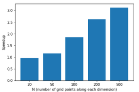
Figure 1: Diffusion equation speedup using AmgX.

When the problem dimension reaches 500 (i.e., 500x500, or 250,000 grid points), the pyamgx wrapper around AmgX speedup is 3x.

Summary

Interpreted languages typified by Python are very quickly becoming popular for science, and Python is already the most popular language for Deep Learning. A number of libraries and extensions have been written for Python, some of which are accelerated with the use of GPUs – but some of which are not.

Ashwin Srinath’s Python interface to Nvidia’s AmgX algebraic multigrid library that runs on GPUs has a wide range of applicability in fluid flow, physics, and astrophysics.

He applied the Python interfaces to the problem of fluid diffusion with the use of FiPy and showed how easy it was to use the AmgX library through the Python interface to get a 3.0x speedup.