
The Python Data Analysis Library, or Pandas, is built on top of the fast math library NumPy and makes analysis of large volumes of data an easy and efficient experience.
Pandas: Data Analysis with Python
In an age when laptops are more powerful and offer more features than high-performance servers of only a few years ago, whole groups of developers are discovering new opportunities in their data. However, companies without a large development department still lack the manpower to develop their own software and tailor it to suit their data. The pandas Python library provides pre-built methods for many applications.
Panda Analysis
The Pandas acronym comes from a combination of panel data, an econometric term, and Python data analysis. It targets five typical steps in the processing and analysis of data, regardless of the data origin: load, prepare, manipulate, model, and analyze.
The tools supplied by Pandas save time when loading data. The library can read records in CSV (comma-separated values), Excel, HDF, SQL, JSON, HTML, and Stata formats; Pandas places much emphasis on flexibility, for example, in handling disparate cell separators. Moreover, it reads directly from the cache or loads Python objects serialized in files by the Python pickle module.
The preparation of the loaded data then follows. Records are deleted, if erroneous entries are found, or set to default values, as well as normalized, grouped, sorted, transformed, and otherwise adapted for further processing. This preparatory work usually involves labor-intensive activities that are very much worth standardizing before you start interpreting the content.
The interesting Big Data business starts now, with computing statistical models that, for example, allow predictions of future input using algorithms from the field of machine learning.
NumPy Arrays
For a long time, the main disadvantage of interpreted languages like Python was the lack of speed when dealing with large volumes of data and complex mathematical operations. The Python NumPy (Numerical Python) library in particular takes the wind out of the sails of this allegation. It loads its data efficiently into memory and integrates C code, which compiles at run time.
The most important data structure in NumPy is the N-dimensional array, ndarray. In a one-dimensional case, ndarrays are vectors. Unlike Python lists, the size of NumPy arrays is immutable; its elements are of a fixed type predetermined during initialization – by default, floating-point numbers.
The internal structure of the array allows the computation of vector and matrix operations at considerably higher speeds than in a native Python implementation.
The easiest approach is to generate NumPy arrays from existing Python lists:
np.array([1, 2, 3])
The np stands for the module name of NumPy, which by convention – but not necessarily – is imported using:
import numpy as np
Multidimensional matrices are created in a similar way, that is, with nested lists:
np.array([[1, 2, 3], [4, 5, 6]])
If the content is still unknown when you create an array, np.zeros() generates a zero-filled structure of a predetermined size. The argument used here is an integer tuple in which each entry represents an array dimension. For one-dimensional arrays, a simple integer suffices:
array2d = np.zeros((5,5))
array1d = np.zeros(5)
If you prefer 1 as the initial element, you can create an array in the same way using np.ones().
The use of np.empty() is slightly faster because it does not initialize the resulting data structure with content. The result, therefore, contains arbitrary values that exist at the storage locations used. However, they are not suitable for use as true random numbers.
The syntax of np.empty() is the same as np.zeros() and np.ones(). All three functions also have a counterpart with the suffix _like (e.g., np.zeros_like()). These methods copy the shape of an existing array, which is passed in as an argument and creates the basis of a new data structure of the same dimensions and the desired initial values.
The methods mentioned also accept an optional dtype argument. As a value, it expects a NumPy data type (e.g., np.int32, np.string_, or np.bool), which it assigns to the resulting array instead of the standard floating-point number. In the case of np.empty(), this again results in arbitrary content.
Finally, the NumPy arange() method works the same way as the Python range() command. If you specify an integer argument, it creates an array of that length, initializing the values with a stepped sequence:
In: np.arange(3)
Out: array([0, 1, 2])
The arange() method optionally takes additional arguments, like its Python counterpart range(). The second argument defines a final value, whereas the first is used as the seed for the sequence. A third argument optionally changes the step size. For example, use
In: np.arange(3, 10, 2)
Out: array([3, 5, 7, 9])
to generate a sequence from 3 to 10 with a step size of 2.
Basic Arithmetic Operations
NumPy allows many operations applied against all elements of an array without having to go through Python-style loops. Known mathematical operators are used (e.g., + for simple addition). The basic rule is that, if two uniform arrays exist, the operator manipulates elements at the same position in both arrays; however, if you add a scalar (i.e., a number) to an array, NumPy adds that number to each array element:
In: np.array([1,2,3]) + np.array([3,2,1])
Out: array([4, 4, 4])
In: np.array([1,2,3]) + 1
Out: array([2, 3, 4])
Multiplication, division, subtraction, and power calculations with ** work in the same way. Additionally, NumPy has some universal functions for further calculations, such as sqrt() and square(), which compute the square root or the power of 2 for each content element of an array.
List and Dictionary Methods
Access to the elements of a NumPy array involves indexes and slices as in Python. The first element is returned by array[0], whereas array[2] returns the first two. For multidimensional arrays, a comma-separated argument list accesses the individual dimensions, such as array[0,2]. Again, slices allow the extraction of areas.
In addition to the list functions, NumPy also supports set operations. The unique() method only outputs the different elements of an array and, in practice, creates a set. Intersections and union sets of one-dimensional arrays with intersect1d() and union1d() are also at hand.
Serial Pandas
Pandas introduces other data structures based, directly or indirectly (Pandas v.013) on NumPy arrays text that combine the efficiency of NumPy with simple craftsmanship. First up is the Series object, a one-dimensional NumPy array; however, it does have some additional methods and attributes. Creating a Series object is much like creating a NumPy array:
s = pd.Series([1, 2, 3])
One of the enhancements compared with NumPy arrays involves the indices that contain the Series objects. If they are not defined explicitly, they exist as a list of consecutive numbers. The indices can also be strings or any other data type:
Series([1, 2, 3], index=['a', 'b', 'c'])
Now you can retrieve the elements much like a Python dictionary (e.g., with s['a']). Pandas takes this into account and allows the initialization of a Series object directly from a Python dictionary:
Series({'a': 1, 'b': 2, 'c': 3})In this use case, too, you can pass in a list separately as an index argument so that only those elements that exist in the index make their way from the dictionary to the resulting Series object. Conversely, Pandas initializes values for indexes that are missing in the dictionary, as non-existing (NaN). In the following case, the entry for 'D' is missing from the results, whereas 'C' is initialized without a value.
In: Series({'a': 1, 'b': 2, 'd': 4}, index=['a', 'b', 'c'])
Out:
a     1
b     2
c   NaN
dtype: float64
Indexes are separate Pandas data objects that are generally immutable. However, they can be replaced with the reindex() method. It accepts a list as an argument, as well as the index argument, when initializing a Series.
Again, Pandas pads nonexistent values with NaN and removes values that no longer exist in the new index. Instead of NaN, you use the fill_value argument to specify different default values. To fill empty rows with 0, use:
s.reindex(['d', 'e', 'f'], fill_value=0)
The s indicates a previously generated Series object.
Framed
Pandas uses the DataFrame class to implement two-dimensional structures. The DataFrame object is again initialized in the same ways as a Series by defining the rows via a dictionary in which each key contains a value comprising a list of elements:
DataFrame({'a': [1, 2], 'b': [3, 4]})An optional index list determines the indices, as for a Series.
In: DataFrame({'a': [1, 2], 'b': [3, 4]}, columns=['a', 'c'], index=['top', 'bottom'])
Out:
        a    c
top     1  NaN
bottom  2  NaN
Columns that are not in the columns list are dropped. However, Pandas again initializes undefined columns with NaN. Access to a column in a DataFrame is again via dataframe['a'], as for a dictionary. Additionally, the columns can be accessed as attributes of a DataFrame object: dataframe.a. If you instead want to address a row, the DataFrame attribute, ix lets you do so: dataframe.ix['top'].
Like Series, the DataFrame object also supports the reindex() method. By default, it references the row labels, but the columns argument replaces the column names in the same way. For both Series and DataFrame objects, the drop() method removes one or more lines. In the first case, you state the desired index as an argument. A list is used to delete multiple rows: s.drop(['b', 'c']).
Files
In the Big Data real world, the data to be analyzed do not usually originate directly with the application that analyzes them. Pandas thus comes with some auxiliary functions that read popular file formats and transfer their contents directly into Pandas data structures: read_csv(), read_table(), and read_fwf(). Figure 1 shows an example of a session with the advanced Python shell, IPython, and a call to read_csv(); Figure 2 shows a curtailed record.
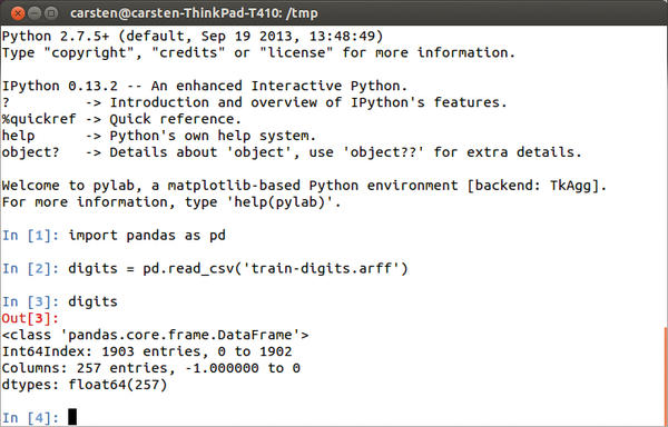 Figure 1: IPython and Pandas for interactive data analysis.
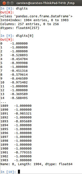 Figure 2: Pandas reads and writes data from and to files and displays the data in a clear-cut way.
These methods expect data sources in tabular form (i.e., one record per line and comma- or tab-separated cells). Arbitrary field separators can be defined with the sep argument in the form of simple strings or regular expressions.
For read_fwf() only, fixed field widths remove the need for field separators; instead, you pass in a list of field widths, stated as the number of characters, or colspecs, stated as the absolute start and end values of each column as a tuple. As a data source, the read methods always expect the first argument to be file names or URLs – or a path.
By default, Pandas reading methods interpret the first line of a file as a header that contains the column names. If you set the argument header=None when calling the method, the first line becomes the first record. In this case, it makes sense to pass in the column names as a list using the names argument.
To save memory and time when processing very large files, the iterator=True argument instructs all the read functions to do the reading chunkwise. Instead of returning the complete file contents, they then return a TextParser object. The size of the read chunks is specified by the chunksize argument. If this argument is set, Pandas automatically sets the iterator to True. Using a TextParser, you can read and process the data line by line in a for loop. The get_chunk() method directly returns the next chuck of the file.
The Series and DataFrame structures make it just as easy to write their content to files. Both have a to_csv() method that expects the output file as an argument; if you instead specify sys.stdout, it passes the data directly to the standard output. The default field separator is the comma, but you can declare an alternative with the sep argument.
Various Formats
Pandas can even process Excel files using the ExcelFile class. Its constructor expects the file path; the resulting ExcelFile uses the parse() method to return DataFrame objects of the individual sheets:
excelfile = pandas.ExcelFile('file.xls')
dataframe = excelfile.parse('Sheet1')
If so desired, Pandas uses the pickle module to store binary format objects on disk. Series and DataFrames, and all other Pandas structures, support the save() helper method for this. It simply expects the output file as an argument. Conversely, the Pandas load() method reads the file and returns the corresponding object.
The data library also adds support for HDF5 (Hierarchical Data Format), which is used, among other programs, by Matlab mathematics software. The advantage is that it can be read efficiently in chunks, even when using compression, so it is particularly suitable for very large data sets.
Pandas uses the HDFStore class to read HDF5 files; the class constructor expects a file name. The resulting object can be read much like a dictionary:
hdf = HDFStore('file.h5')
s1 = hdf['s1']
These calls read the file.h5 HDF file, whose data structure contains a Series object named s1. This is also stored in the s1 variable.
Data!
After reading the data, Pandas applies numerous auxiliary functions to shape them. First, merge() merges two DataFrame objects,
pandas.merge(dataframe1, dataframe2)
here, by combining the columns of two DataFrames on the basis of identical indices by default. If instead you want to use another column to identify the records to be merged, you can use the on argument to specify the relevant name. This of course only works if both data frames contain a like-named column.
Instead of merging records in two objects, concat() concatenates Series or DataFrames. In the simplest case, the concatenation of two Series objects creates a new Series object that lists all the entries in the two source objects in succession. Alternatively, the line
concat([series1, series2, series3], axis=1)
generates a DataFrame from multiple Series objects. In this example, the function concatenates the sources on the basis of the columns (axis=1), instead of line by line (axis=0).
SQL database users are familiar with the concat() functionality from joins. By default, the inner method is used; this generates an intersection of the keys used. Alternatively, you may use the outer (union), left, or right method. With left and right, the result of a merge contains only the keys of the left or right source object, respectively.
On and On
Pandas offers a plethora of auxiliary functions for data manipulation. The DataFrame methods stack() and unstack(), for example, rotate a DataFrame so that the columns become rows and vice versa.
To clean up existing data, Pandas provides drop_duplicates(), which dedupes Series and DataFrame objects. In contrast, replace() searches for all entries with a certain value and replaces the matches with another value:
series.replace('a', 'b')The map() method is more generic: It expects a function or a dictionary and automatically converts the entries of a data object. For example, the following example uses the str.lower() function to convert all entries in a column to lowercase:
dataframe['a'].map(str.lower)
In true Python style, Pandas again allows an anonymous lambda function to be passed in. At this point, you can also appreciate the power of vectorization that NumPy supports. The Series class provides, among other things, a separate str property that does not require line-by-line iteration to process strings. For example:
series.str.contains("ADMIN")finds all entries that contain the ADMIN string.
Future
Pandas offers many data manipulation methods that I was unable to cover in this article and many equally unmentioned arguments that change functions into useful helpers in more or less everyday application cases. Moreover, Pandas uses the plot() method (Figure 3) from the Matplotlib library to visualize DataFrames and Series. The Pandas documentation contains a complete reference (Figure 4).
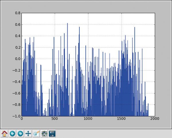 Figure 3: Using Matplotlib to visualize Pandas records.
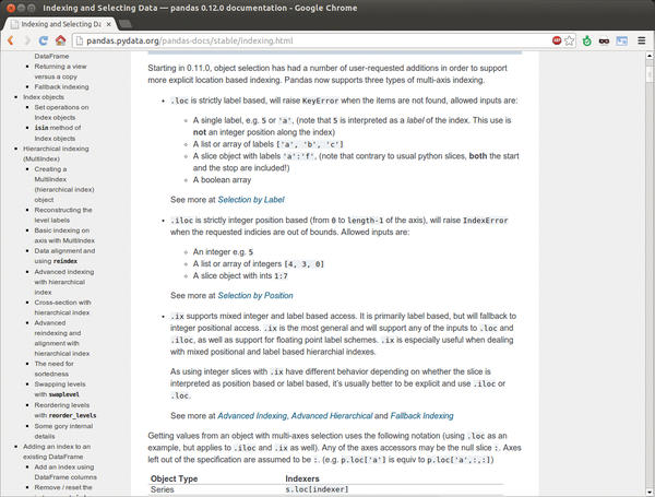 Figure 4: The Pandas documentation lists all of the library’s resources.
The Pandas data library shows that Python is mature enough – mainly thanks to the NumPy foundation – to take on compiled languages in terms of speed, while offering the benefits of intuitive syntax and a variety of interactive shells.