
Understanding how applications perform I/O is important not only because of the volume of data being written and read, but because the performance of some applications is dependent on how I/O is conducted. In this article we profile I/O at the block layer to help you make the best storage decisions.
ioprof, blktrace, and blkparse
Applications are consuming and producing data at an unprecedented rate. In general, you can chose storage that most closely matches the application I/O patterns, make changes to the application to match a fixed storage architecture, or choose a solution in between. Therefore, knowledge of I/O patterns in applications is a critical step toward understanding your storage options.
In the past, I wrote about I/O tracing by looking at I/O patterns the application sends to the system (system calls) with strace. These patterns can reveal a great deal about what the application is doing. However, data moves through a number of levels in the software stack from the application to the actual storage device. strace is useful from the perspective of understanding what the application is requesting in terms of I/O, but it is also useful to look further down the stack to see how the I/O requests appear at the various layers. One layer that is useful to monitor is the block layer, which is near the bottom of the stack and represents what is sent to the drives.
Linux has some excellent tools for tracing I/O request queue operations in the block layer. The tools that come with the kernel are blktrace and blkparse. If you’re not running a kernel before 2.6.16, then these tools should be on your system. On my CentOS 6.5 system, I found them in an RPM named blktrace. These are very powerful tools, but they can be a bit complicated to use; however, a few additional tools can take the blktrace information and present it in a form that mere mortals can understand. One of the tools that fits this bill is the Linux I/O profiler, or ioprof.
ioprof
When I discovered that understanding the output of blktrace was not so easy, I looked around for some “postprocessing” tools and came across ioprof. The website introduces the tool as follows:
The Linux I/O Profiler is an easy-to-use tool that helps administrators reduce server storage bottlenecks by providing significant insight into I/O workloads. While the primary focus of this tool is for use with SSDs, it can be used to identify hotspots coming from RAID arrays, tier storage systems, software and hardware RAID, as well as virtual and hardware logical volumes.
The tool uses blktrace and blkparse to examine block I/O patterns. In particular, the tool provides the following (from the README file):
- I/O histogram – Great for determining size of hot data for SSD caching
- I/O heat map – Useful visualization to “see” where the hot data resides
- I/O size stats – IOPS and bandwidth stats, which are useful for mixed workloads
- Top files (opt) – IDs top accessed files in ext3/ext4 filesystems
- Zipf theta - Estimate of Zipfian distribution theta
Ioprof is written in Perl and is fairly easy to run, but it has to be run as root (or with root privileges).
Ioprof runs in three modes. The first mode simply gathers the data on the block device(s) for later postprocessing. The second mode processes the output, producing an ASCII report and an optional PDF report. The third “live” mode lets you see what’s happening in close to real time. When gathering the data on the block device(s), you can input a single device (e.g., /dev/sdb1) or multiple devices (e.g., /dev/sdb1,/dev/sdc1).
Using ioprof means you don't have to learn the details of blktrace and blkparse, because it collects everything for you and creates the report(s). Iofprof gives you a reasonable idea of what’s happening on the storage device at the block level.
To explore how ioprof works, I decided to apply it to a known benchmark in a test. The example is somewhat arbitrary and won’t likely provide useful information beyond how ioprof works. The benchmark I will use is IOzone.
IOzone Example
The ioprof test ran while I was running iozone three ways: (1) sequential write testing with 1MB record size, (2) sequential read testing with 1MB record size, and (3) random write and read (4KB). In running these tests, I wanted to see what block layer information ioprof revealed.
The system I'm using is my home desktop with the following basic characteristics:
- Intel Core i7-4770L processor (four cores, eight threads, with Hyper-Threading, running at 3.5GHz)
- 32GB of memory (DDR3-1600)
- CentOS 6.5 (updates current as of August 22, 2014)
For testing, I used a Samsung SSD 840 Series drive that has 120GB of raw capacity (unformatted) and is connected via a SATA 3 (6Gbps) connection. The device is /dev/sdb with a single partition (/dev/sdb1) and is formatted ext4 and mounted as /data. I'll summarize the results for each of the three tests below.
IOzone Write
The first test run was the sequential write test using 1MB record sizes:
./iozone -i 0 -c -e -w -r 1024k -s 32g -t 2 -+n > iozone_write_1.out
To gather the block statistics, I ran ioprof in a different terminal window before I ran IOzone, and I wrote the ioprof output to a different filesystem to minimize the impact on the test:
./ioprof.pl -m trace -d /dev/sdb1 -r 660
The ioprof command gathers the data it collected into a TAR file (-m trace). In this case, the tar file defaults to sdb1.tar. The command traces the /dev/sdb1 device (-d /dev/sdb) and gathered data for 660 seconds (-r 660). The amount of time was a bit longer than the IOzone run, but nothing else was done with the storage device. One of the cool ioprof features is that, while it is running, it shows a time counter so you know how much time is remaining before it stops.
After collecting the data, it was postprocessed (-m post) with:
./ioprof.pl -m post -t sdb1.tar
The ASCII output without the heat map is shown in Listing 1.
Listing 1: IOzone Write
[root@home4 ioprof-master]# ./ioprof.pl -m post -t sdb1.tar
./ioprof.pl (2.0.4)
Unpacking sdb1.tar.  This may take a minute.
lbas: 234436482 sec_size: 512 total: 111.79 GiB
Time to parse.  Please wait...
Finished parsing files.  Now to analyze
Done correlating files to buckets.  Now time to count bucket hits.

--------------------------------------------
Histogram IOPS:
2.2 GB 10.2% (10.2% cumulative)
4.5 GB 7.8% (17.9% cumulative)
6.7 GB 6.8% (24.7% cumulative)
8.9 GB 6.3% (30.9% cumulative)
11.2 GB 5.9% (36.9% cumulative)
13.4 GB 5.7% (42.6% cumulative)
15.7 GB 5.4% (48.0% cumulative)
17.9 GB 5.2% (53.2% cumulative)
20.1 GB 4.9% (58.0% cumulative)
22.4 GB 4.5% (62.5% cumulative)
24.6 GB 4.1% (66.7% cumulative)
26.8 GB 3.8% (70.5% cumulative)
29.1 GB 3.2% (73.7% cumulative)
31.3 GB 3.0% (76.6% cumulative)
33.5 GB 2.8% (79.4% cumulative)
35.8 GB 2.6% (82.0% cumulative)
38.0 GB 2.4% (84.4% cumulative)
40.3 GB 2.2% (86.6% cumulative)
42.5 GB 2.0% (88.6% cumulative)
44.7 GB 1.8% (90.4% cumulative)
47.0 GB 1.6% (92.1% cumulative)
49.2 GB 1.5% (93.6% cumulative)
51.4 GB 1.3% (94.9% cumulative)
53.7 GB 1.2% (96.1% cumulative)
55.9 GB 1.0% (97.1% cumulative)
58.1 GB 0.8% (98.0% cumulative)
60.4 GB 0.7% (98.7% cumulative)
62.6 GB 0.5% (99.2% cumulative)
64.9 GB 0.4% (99.7% cumulative)
67.1 GB 0.3% (99.9% cumulative)
68.3 GB 0.1% (100.0% cumulative)
--------------------------------------------
Approximate Zipfian Theta Range: 0.0348-1.4015 (est. 0.5043).
Trace_files: 0
Stats IOPS:
"4K WRITE" 100.00% (223855533 IO's)
Stats BW:
"4K WRITE" 100.00% (853.94 GiB)
This heatmap can help you 'see' hot spots.  It is adjusted to terminal size, so each square = 10.00 MiB
The PDF report may be more precise with each pixel=1MB
Heatmap Key: Black (No I/O), white(Coldest),blue(Cold),cyan(Warm),green(Warmer),yellow(Very Warm),magenta(Hot),red(Hottest)
Notice at the end of the output that all of the writes were 4KB data sizes. Even though I requested 1MB record sizes when running IOzone, the data is broken into 4KB chunks once it reaches the block layer.
Ioprof produces a very impressive ASCII heat map by using each character cell on the terminal screen as a “bucket”, where the bucket defaults to 10MB. Each cell is colored and a number is also put in the cell. The ASCII heat map in Figure 1 is from a screen capture when I ran the postprocessing for this test.
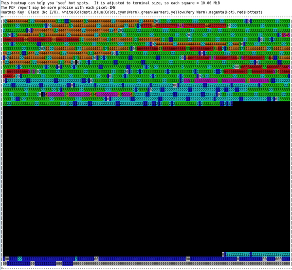 Figure 1: ASCII heat map of blocks during IOzone write testing.
Starting with the first 1MB of the drive, the first ASCII cell represents the first 10MB block, the next ASCII cell in the row is the second 10MB block, and so. At the end of the row, the map wraps.
The key appears above the chart. The black cells had no I/O activity during the run. White cells (they look sort of gray) had the lowest I/O levels and are denoted with a 0 in the cell. Blue, still fairly low I/O, is denoted with a 1. Cyan is the next warmer color with slightly higher levels of I/O and denoted with a 2. Green (3), yellow or orange (4), magenta (5), and red (6 or 7) follow in increasing order. If you ignore black, the scale has seven colors with eight levels of I/O intensity (0–7), but with two levels in red cells.
From the heat map, you can see the concentration of block activity for the drive (remember that it is an SSD drive). Of interest in this test is the good bit of write activity on the first 40% of the drive and the small amount of activity on the last part of the drive. In the case of an SSD, you don’t want to see hot spots if you can help it, because that will use up the rewrite cycles at a faster rate.
IOzone Read
The second test was the sequential read test option in IOzone:
./iozone -i 1 -c -e -w -r 1024k -s 32g -t 2 -+n > iozone_read_1.out
The ioprof command run before the iozone command was::
./ioprof.pl -m trace -d /dev/sdb1 -r 200
The ioprof command is very similar to the one used for the write test, except it gathered data for just 200 seconds (-r 200), which covered the time it took to run the iozone test.
After the data was collected it was postprocessed with the command:
./ioprof.pl -m post -t sdb1.tar
The ASCII output without the heat map is shown in Listing 2.
Listing 2: IOzone Read
[root@home4 ioprof-master]# ./ioprof.pl -m post -t sdb1.tar
./ioprof.pl (2.0.4)
Unpacking sdb1.tar.  This may take a minute.
lbas: 234436482 sec_size: 512 total: 111.79 GiB
Time to parse.  Please wait...
Finished parsing files.  Now to analyze
Done correlating files to buckets.  Now time to count bucket hits.

--------------------------------------------
Histogram IOPS:
2.2 GB 7.6% (7.6% cumulative)
4.5 GB 6.8% (14.4% cumulative)
6.7 GB 6.4% (20.7% cumulative)
8.9 GB 5.9% (26.6% cumulative)
11.2 GB 5.5% (32.1% cumulative)
13.4 GB 5.2% (37.3% cumulative)
15.7 GB 4.9% (42.2% cumulative)
17.9 GB 4.7% (46.9% cumulative)
20.1 GB 4.3% (51.2% cumulative)
22.4 GB 4.2% (55.3% cumulative)
24.6 GB 4.1% (59.4% cumulative)
26.8 GB 3.7% (63.0% cumulative)
29.1 GB 3.6% (66.7% cumulative)
31.3 GB 3.6% (70.3% cumulative)
33.5 GB 3.2% (73.5% cumulative)
35.8 GB 3.1% (76.6% cumulative)
38.0 GB 3.1% (79.8% cumulative)
40.3 GB 2.8% (82.5% cumulative)
42.5 GB 2.6% (85.2% cumulative)
44.7 GB 2.6% (87.7% cumulative)
47.0 GB 2.4% (90.1% cumulative)
49.2 GB 2.1% (92.2% cumulative)
51.4 GB 2.0% (94.2% cumulative)
53.7 GB 1.6% (95.8% cumulative)
55.9 GB 1.4% (97.2% cumulative)
58.1 GB 0.9% (98.0% cumulative)
60.4 GB 0.5% (98.6% cumulative)
62.6 GB 0.5% (99.1% cumulative)
64.9 GB 0.5% (99.6% cumulative)
67.1 GB 0.4% (100.0% cumulative)
67.6 GB 0.0% (100.0% cumulative)
--------------------------------------------
Approximate Zipfian Theta Range: 0.0087-1.0291 (est. 0.3942).
Trace_files: 0
Stats IOPS:
"44K READ" 3.02% (109768 IO's)
"84K READ" 3.02% (109745 IO's)
"128K READ" 93.53% (3394859 IO's)
Stats BW:
"44K READ" 1.07% (4.61 GiB)
"84K READ" 2.05% (8.79 GiB)
"128K READ" 96.66% (414.41 GiB)
This heatmap can help you 'see' hot spots.  It is adjusted to terminal size, so each square = 10.00 MiB
The PDF report may be more precise with each pixel=1MB
Heatmap Key: Black (No I/O), white(Coldest),blue(Cold),cyan(Warm),green(Warmer),yellow(Very Warm),magenta(Hot),red(Hottest)
Notice that three read sizes were used in the block layer: 44, 84, and 144KB, which is a bit different from the sequential write tests. The corresponding ASCII heat map is shown in Figure 2.
 Figure 2: ASCII heat map of blocks during IOzone read testing.
From the heat map you can see the concentration of block activity for the SSDS drive. Of interest in this test again is the good bit of read activity on the first 40% of the drive and a small amount of activity on the last part of the drive – although it is larger than during the sequential write test.
IOzone Random Small Read and Write
The third test I ran was the random read and write test with small record sizes and a smaller total file size (a kind of random IOPS run):
./iozone -i 2 -w -r 4k -I -O -w -+n -s 4g -t 2 -+n > iozone_random_1.out
The total file size for this test was much smaller than the others (4GB compared with 32GB). The ioprof command run before the iozone command was:
./ioprof.pl -m trace -d /dev/sdb1 -r 330
The command is similar to that used for the write test, except it gathered data for just 330 seconds (-r 330), which covered the time it took to run the IOzone test.
After the data was collected it was postprocessed:
./ioprof.pl -m post -t sdb1.tar
The ASCII output without the heat map is shown in Listing 3.
Listing 3: IOzone Random Small Read and Write
[root@home4 ioprof-master]# ./ioprof.pl -m post -t sdb1.tar
./ioprof.pl (2.0.4)
Unpacking sdb1.tar.  This may take a minute.
lbas: 234436482 sec_size: 512 total: 111.79 GiB
Time to parse.  Please wait...
Finished parsing files.  Now to analyze
Done correlating files to buckets.  Now time to count bucket hits.

--------------------------------------------
Histogram IOPS:
2.2 GB 28.3% (28.3% cumulative)
4.5 GB 27.9% (56.2% cumulative)
6.7 GB 27.6% (83.9% cumulative)
8.6 GB 16.1% (100.0% cumulative)
--------------------------------------------
Approximate Zipfian Theta Range: 0.0001-1.1051 (est. 0.2888).
Trace_files: 0
Stats IOPS:
"4K READ" 56.16% (18915462 IO's)
"4K WRITE" 43.84% (14764645 IO's)
Stats BW:
"4K READ" 56.16% (72.16 GiB)
"4K WRITE" 43.84% (56.32 GiB)
This heatmap can help you 'see' hot spots.  It is adjusted to terminal size, so each square = 10.00 MiB
The PDF report may be more precise with each pixel=1MB
Heatmap Key: Black (No I/O), white(Coldest),blue(Cold),cyan(Warm),green(Warmer),yellow(Very Warm),magenta(Hot),red(Hottest)
Notice that for this test all of the reads and writes were 4KB. Because this was a random test, it appears that writes or reads were unable to be combined. This tells me that the block layer saw exactly what I want to test – random 4KB performance (roughly IOPS).
The ASCII heat map for this test is shown Figure 3. All of the I/O was done at the end of the drive, except for a very tiny part at the very beginning (maybe the output from iozone), which is different from the sequential testing (I’m not sure why).
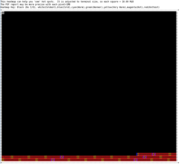 Figure 3: ASCII heat map of blocks during IOzone random read and write testing.
PDF Output from ioprof
One of the unique capabilities of ioprof is the ability to create a nice PDF report of the postprocessing with good charts. I want to present just a couple of snippets from one of these reports so you can see what some of the charts look like.
To use the PDF feature, you need to install TeX (assuming LaTeX) and a tool called pdf2latex. You also need gnuplot installed and “terminal png.” Sometimes these tools are already present, but you might have to install them yourself. In my case for CentOS 6.5, I found pdflatex in a Yum group named texlive-latex. The binary is called /usr/bin/pdflatex, which is a symlink to /usr/bin/pdftex.
For this article I postprocessed the sequential write test results but added the PDF option (-p):
./ioprof.pl -m post -t sdb1.tar -p
This produces the same ASCII output along with the PDF. Figures 4–6 are the three plots from the PDF. Figure 4 shows the percentage of total I/O that fell into each part of the block device.
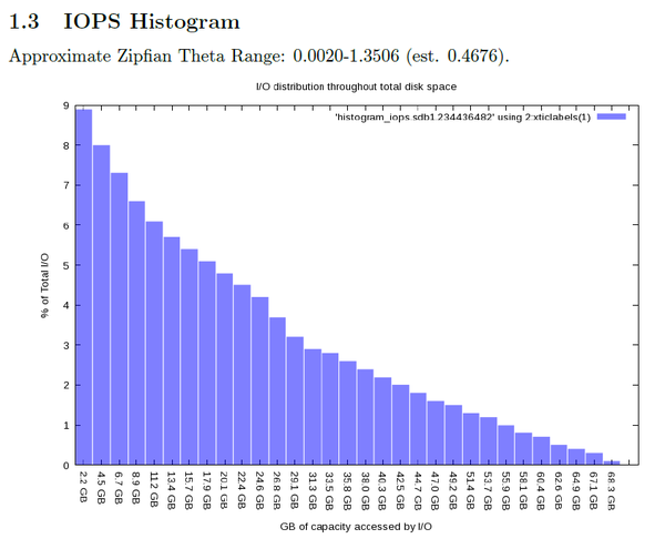 Figure 4: PDF IOPS histogram during IOzone write test.
The IOPS heat map in Figure 5 is more detailed than the ASCII chart, using 1MB buckets instead of 10MB buckets.
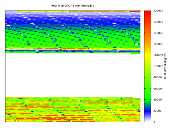 Figure 5: PDF IOPS heat map chart during IOzone write test.
Figure 6 is a chart of the IOPS statistics (size of I/O request).
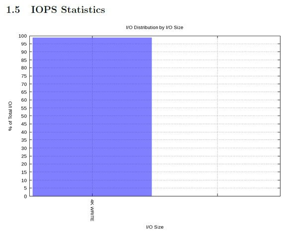 Figure 6: PDF IOPS statistics during IOzone write test.
For this example, it just shows that the test used 4KB writes, but you can see how this chart could be really useful when you have a number of applications performing different types of I/O.
Summary
Understanding how data makes its way from the application to storage devices is key to understanding how I/O works. With this knowledge, you can make much better decisions about storage design, storage purchases, or whether to redesign your application. Monitoring the lowest level of the I/O stack, the block driver, is a crucial part of this overall understanding of I/O patterns.
Linux comes with a couple of tools, blktrace and blkparse, for tracing activity at the block level; however, they can be difficult to use and require a little finesse. A nifty tool named ioprof uses these tools to produce a very useful report of I/O patterns at the block level that includes histograms, heat maps, and I/O size stats. You can run ioprof in a data gathering mode that collects data for later postprocessing, a “live” mode that lets you watch developments in real time, and a postprocessing mode that produces some really useful output. The ASCII IOPS heat map charts can be very useful for a quick evaluation of I/O behavior, and the PDF version of the report has some great charts.
If you are interested in understanding the I/O patterns of your applications, understanding what is happening at the block level is fairly important. Ioprof is a new tool that makes understanding block level I/O very easy.