
Most of the time people turn to data compression to save storage space, but reducing precision can be a useful technique.
Saving Storage Space with Reduced Precision
Since the beginning of computing, people have been trying to save storage space, which never seems to be enough, especially for massive datasets (e.g., for artificial intelligence). Almost 100% of the people I know use compression tools to save space. Although this method can work on some file types, it’s not really useful for binary files.
After trying to compress files, users classically give up and ask for more storage space. Sometimes they get a little desperate and start using USB sticks or external drives or try to build their own “inexpensive” storage boxes or find ways to stack data in the cloud (e.g., storing photos or trying to use Gmail for storing data). By and large, though, people run something like gzip and just ask for more space.
AI has really driven home the message that those in HPC don’t need to compute everything in double-precision floating-point format (FP64). For some problems, you can use single precision (FP32) and compute faster and use less storage space. Reducing precision from FP64 to FP32 can halve the needed storage space.
Although I’m not sure of the true number, I believe a large percentage of HPC users think that if they compute with a certain representation (number of bits), they need to store data in that same representation. But is this necessary?
I think most people understand that modern processors have different numerical representations (FP64, FP32, FP16, Bfloat16, FP8, TF32, INT16, INT8, INT4, etc.) that have an effect on how much memory is used and how many bits are used in computations. For many years you saw processors with just a very small number of these representations (maybe two or three?). Now processors can have most or even all of them.
I have worked in computational fluid dynamics (CFD) for a while, and we used FP64 almost exclusively when I was running production code, which means that each value was stored in 64 bits. Way back when, this was quite a bit of space, and even now for large problems, it can be a large amount of space, especially as problem sizes get larger and longer simulations are performed. How can you save space?
Compression
Data compression takes information (data) and uses fewer bits to represent the exact same data without losing any accuracy or precision. This method is referred to as “lossless” compression. For scientific data, virtually all of the current compression tools are lossless. In 2021 I wrote an article listing common tools for lossless compression. Note that some of these tools can even be run in parallel to decrease the amount of time to compress or uncompress the data.
Depending on the data, compression can save you a great deal of data storage or not very much at all. An example of “easy-to-compress” data is text. An example of “difficult-to-compress” data is binary data. From a Stack Exchange question, an article was mentioned that showed data compression ratios of two to four times.
The typical user uses compression tools not only to save space, but also not to lose data and keep the precision the same (i.e., lossless compression). In some cases, the image format allows for the loss of some data without affecting the original image, not really affecting the overall image quality from the perspective of the human eye, but saving space. This method is termed lossy compression.
Naturally users want to retain all of their data if they compress, but have you thought whether you need to retain the precision of the data, particularly output data? If you took an output data file that is in FP64 and changed it to FP32, the data file will be half the size. Are you losing anything important by reducing the data size? I don’t believe you can have a general answer for that question, but it definitely deserves consideration given the amount of data some people use, create, and archive.
Reducing Precision to Save Storage
Reducing the precision of your data can be accomplished in several ways, and a single method will not answer for all problems and data types in all situations. Ultimately, the choice is up to you, but I suggest you investigate the possibilities.
Type Casting
One way to reduce precision after computations are finished is to “type cast” the data you want to save from a higher precision to a lower precision before saving the data and while the application is still running. Simple code to read in the data at full precision and write it out at a lower precision also works. (Don’t forget to delete the data in full precision or you are not saving space.)
The following example takes a double-precision number and converts it to single precision, which boils down to a “rounding problem” of something like addition, multiplication, and so on. The explanation of this process is fairly well treated online. You must follow five different rules for rounding:
- Round to the nearest value, ties round to even
- Round to the nearest value, ties round away from zero
- Directed rounding toward 0
- Directed rounding toward +infinity
- Directed rounding toward −infinity
Converting from FP64 to FP32 uses these rules until the proper FP32 representation is achieved.
Normalize
One way to normalize the data is to use a standard score, which is the number of standard deviations the raw score is from the mean and is commonly known as the z-score,
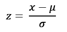 Figure 1: z-Score formula.
where x is the list of raw data, µ is the mean, σ is the standard deviation, and z is the normalized number of standard deviations from the mean value. The z-score can be a positive or negative number.
After computing z, you can examine the range of values. If the range fits within the range of a reduced-precision variable, you can save the z values, as well as µ and σ in their original precision. This method saves storage space with the penalty of storing two extra values (µ and σ) that need to be stored at the higher precision. If you need to “rehydrate” your data to actual values instead of z-scores, you can reverse the process with the advantage of having higher precision values for µ and σ.
Converting your data to z-scores transforms that distribution of values in a couple of ways. First, it takes very, very large positive or negative numbers and reduces their values, which pushes the values away from the upper and lower limits of the current precision. If you have a large distribution of values (i.e., a very large range of values), then this method will reduce the data values.
Second, values close to the median move very close to zero, perhaps requiring large precision to represent them accurately. For example, if a data point has the value 1.000001 and the stand deviation is 1.0, the resulting z-score is then 0.000001.
Overall, the effect is that some of the data might need to be represented by the current precision and not reduced precision. However, you can use the z-scores to reduce the precision of the entire dataset or a large part of the data set.
After converting the data to z-scores you can examine the distribution of values with respect to the range of single-precision values. Some data values fall out of the bound of single precision. You can save the data values within the single-precision bound as single precision and save the outlying values in double precision. This method can save storage space if not too many outliers have to be stored in double precision.
Another option is to type cast the outlying values to single precision and store everything as single precision except the mean and standard deviation. However, you have to make the decision about type casting to a lower precision.
In some cases quite a few z values can be outside the range of single precision. When this happens, you can either look for another method of converting the data to a lower precision (e.g., double precision to single precision), or you could choose to normalize the data and accept the reduction in precision in the outliers. This decision is totally up to you.
Other normalization techniques are like standard scores. One example is to use the range of values in x instead of the stand deviation as the divisor:
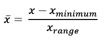 Figure 2: Range normalization formula.
This normalization may or may not be useful because it produces numbers in the range 0–1. You have to decide whether this method works for normalizing your data and saving it at a lower precision.
You can probably think of other normalizations, some of which might be really weird, but the goal is take your data and try to put all of it in the range of the lower precision, so information is not lost or the amount of information lost is minimized when saving to single precision.
Truncate Data to Reduce Precision
Another, perhaps drastic, idea – but one to be considered – is to truncate the higher precision data to obtain lower precision. This method is different from type casting (rounding the data). Truncate means just to drop the specific decimal portion of the value. For example, a value of 4.2 rounds to 4 and truncates to 4 as well. A value of 2.99 truncates to 2 and rounds to 3.
A simple illustration of truncation is shown in Figure 3. At the top of the figure is a decimal number. Below, the scissors indicate where a decimal number is being truncated. Effectively, it just cuts off everything to the right of the scissors. At the bottom of the figure is the resulting truncated decimal number.
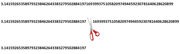 Figure 3: Simple illustration of truncation.
To reduce double precision to single precision by truncation, you cut off the decimal values until the value falls within the single-precision limits.
For example, if I want to reduce the value 7.726 to two decimal places, rounding (type casting) gives me 7.73, whereas truncating yields 7.72.
I haven’t had a reason to truncate, so I typically just round numbers until I achieve the precision, or number of decimal places, I want. If you are interested in truncation, please look around for articles about using it and its pluses and minuses.
Type Casting Examples
In these examples of type casting I use Python and Fortran, but you can choose whatever language you like because the concepts are the same, although the details will vary.
Python Example
HPC typically uses NumPy, so I will be showing how to do type casting with this library. A NumPy array is referred to as an ndarray data type, which you specify on creation. Table 1 lists the data types you can use (from an nkmk blog).
Table 1: NumPy Data Types
| dtype | Character code | Description | |
|---|---|---|---|
| int8 | i1 | 8-bit signed integer | |
| int16 | i2 | 16-bit signed integer | |
| int32 | i4 | 32-bit signed integer | |
| int64 | i8 | 64-bit signed integer | |
| uint8 | u1 | 8-bit unsigned integer | |
| unit16 | u2 | 16-bit unsigned integer | |
| unit32 | i4 | 32-bit unsigned integer | |
| unit64 | i8 | 64-bit unsigned integer | |
| float16 | f2 | 16-bit floating-point | |
| float32 | f4 | 32-bit floating-point | |
| float64 | f8 | 64-bit floating-point | |
| float128 | f16 | 128-bit floating-point | |
| complex64 | c8 | 64-bit complex floating-point | |
| complex128 | c16 | 128-bit complex floating-point | |
| complex256 | c32 | 256-bit complex floating-point | |
| bool | ? | Boolean (True or False) | |
| unicode | U | Unicode string | |
| object | O | Python object | |
A simple example from nkmk creates a float64 data type (64-bit floating-point number):
import numpy as np a = np.array([1, 2, 3], dtype=np.float64) |
Expanding on the previous example, you can use NumPy to type cast from float64 to float32 (Listing 1) with the astype function. Notice that I copied the float64 array (a) to the float32 array (b). If you were to do a simple assignment operation (e.g., b = a) and then assign the data type, you would change the data type of variable a.
Listing 1: Change Type Cast
import numpy as np

N=100
a = 100.0*np.random.random((N,N))
a.astype(np.float64)
print("a[5,5] = ",a[5,5]," type = ",a[5,5].dtype)
np.save('double', a)

b = np.copy(a)
b = b.astype(np.float32)
print("b[5,5] = ",b[5,5]," type = ",b[5,5].dtype)
np.save('float', b)

print("Difference = ",a[5,5]-b[5,5])
|
Some output from this simple example is:
a[5,5] = 37.6091660659823 type = float64 b[5,5] = 37.609165 type = float32 Difference = 8.743319099835389e-07 |
Note the difference between the float64 and float32 values. The difference is approximately 8.74e−7. Is this difference important given the magnitude of the two values? Again, there is no general rule as to whether the difference is important or not. You have to make that decision but don’t minimize asking that question.
In terms of storage space, the double-precision file was approximately 80KB, and the single-precision file only 40KB (half the space). Both are binary files. For computations with a great deal of data, the difference in storage space can be important, which should be a consideration as you determine whether reduction of precision in the solution will lose much (if any) precision needed by the problem.
Fortran Example with 2D Array
You can also reduce precision in Fortran with specific type conversion functions that allow you to change a variable or an array from one type to another:
- real
- int
- dble
- complex
In the next example of simple Fortran code (Listing 2), a 2D array of random values with a size of 100 is created of double-precision values, and a second array is created from the first, but in “real” precision (single precision) with the real function. Although probably not proper Fortran (I didn’t even check the values of the return from the allocated function), it should get my point across.
Listing 2: Fortran Type Conversion
    program fortran_test_1
    implicit none

    double precision, dimension(:,:), allocatable :: a
    double precision :: x
    real, dimension(:,:), allocatable :: b
    integer :: n, i, j, ierr

!------------------------------------------------------------------
    n = 100

    allocate(a(n,n), stat=ierr)
    allocate(b(n,n), stat=ierr)

    call random_seed()

    do j =1,n
        do i=1,n
            call random_number(x)
            a(i,j) = 10.0d0*x
        end do
    end do
    write(*,*) "a(5,5) = ",a(5,5)

    b = real(a)
    write(*,*) "b(5,5) = ",b(5,5)

    open(unit=1, form="unformatted")
    write(1) a
    close(1)

    open(unit=2, form="unformatted")
    write(2) b
    close(2)

    end program
The compiled code outputs the value of element (5,5) for both the double-precision and real arrays:
./fortran_test1 a(5,5) = 9.9179648655938202 b(5,5) = 9.91796494 |
Notice how the real conversion function rounded the value.
A second part of the code writes each array in binary to a file. After running the code, I listed the files in the directory to check their sizes (Listing 3). Notice that the single-precision file fort.2 is half the size of the double-precision file fort.1, which is what I wanted.
Listing 3: File Sizes
$ ls -sltar
total 152
 4 drwxr-xr-x 56 laytonjb laytonjb 4096 Jun 7 15:34 ..
 4 -rw-rw-r-- 1 laytonjb laytonjb 731 Jun 7 15:40 fortran_test1.f90
20 -rwxrwxr-x 1 laytonjb laytonjb 17280 Jun 7 15:40 fortran_test1
40 -rw-rw-r-- 1 laytonjb laytonjb 40008 Jun 7 15:40 fort.2
80 -rw-rw-r-- 1 laytonjb laytonjb 80008 Jun 7 15:40 fort.1
 4 drwxrwxr-x 2 laytonjb laytonjb 4096 Jun 7 15:40 .
Summary
Imagine having several complex massive (in the gigabyte or terabyte range) 3D arrays. If you don’t need all of the precision, you can write the arrays to files with single precision and save storage space. Of course, the big “if” in that sentence is whether you can lose the precision without a bad effect. The choice is up to you, but I believe it is worthwhile at least trying the concept with some of your code and datasets to judge the outcome for yourself.