
In the second article of this three-part series, we look at simple write examples in Fortran 90 and track the output with strace to see how it affects I/O patterns and performance.
Understanding I/O Patterns with strace, Part II
I’ve written articles in the past about I/O patterns and examined them using strace. This type of information comes from the perspective of the application – that is, what it sends to the OS. The OS then takes these requests and acts on them, returning a result to the application. Understanding the I/O pattern from an application's perspective allows you to focus on that application. You can then switch platforms or operating systems or distributions or even tune the OS, with an understanding of what your application requests from the OS.
The choice of language and compiler or interpreter has a great deal of influence on the resulting I/O pattern, which will be different when using C than when using Fortran, Python, and so on. In a series of three articles, I use three languages that are fairly common in HPC to illustrate these differences: C, Fortran 90, and Python (2.x series). I run the examples on a single 64-bit system with CentOS 6.2 using the default GCC compilers, GCC and GFortran (4.4.6),and the default Python (2.6.6).
With the use of a simple example in each language, I’ll then vary the number of data type elements to get an increasing amount of I/O. The strace output captured when the application is executed will be examined for the resulting I/O. By varying the number of elements, my goal is to see how the I/O pattern changes and perhaps better understand what is happening.
In a previous article, I used strace to help understand the write I/O patterns of an application written in C. Now, I want to do the same thing with an application written in Fortran 90. My goal is to understand what is happening in regard to the I/O and even how I might improve it by rewriting the application (tuning).
Fortran 90
A common language in the HPC world is Fortran. The default version of Fortran commonly used today is Fortran 90, even though more current versions (Fortran 95, Fortran 2003, and even Fortran 2008) are available. I took the C code in the previous article (Listings 2C and 3C) and rewrote it in Fortran 90. Although the code is probably not ideal, and purists will likely chastise me, itshould serve to illustrate my point.
The Fortran code uses binary (non-human-readable) or unformatted output. In Fortran, unformatted files have a 4-byte record written before and after the data. Therefore, a 16-byte record would actually write 24 bytes (4 bytes before the record, the 16-byte record, and 4 bytes after the record). With unformatted I/O, that means a 50% increase in size if I write a single 16-byte record. However, I can use a much larger record size, so the increased need for storage space won’t be quite so pronounced.
A quick translation of the “one-by-one” C code in Listing 2C is translated into Fortran 90 (F90) in Listing 1F.
Listing 1F: F90 Code Example with Output in Loop (One-by-One)
 1    program ex1
 2
 3    type rec
 4       integer :: x, y, z
 5       real :: value
 6    end type rec
 7
 8    integer :: counter
 9    integer :: counter_limit
10    integer :: ierr
11
12    type (rec) :: my_record
13
14    counter_limit = 2000
15
16    ierr = -1
17    open(unit=8, file="test.bin", status="replace", &
18         action="readwrite", form="unformatted", &
19         iostat=ierr)
20    if (ierr > 0) then
21       write(*,*) "error in opening file! Stopping"
22       stop
23    else
24       do 10 counter=1,counter_limit
25          my_record%x = counter
26          my_record%y = counter + 1
27          my_record%z = counter + 2
28          my_record%value = counter * 10.0
29          write(8) my_record
30 10    continue
31    endif
32
33    close(8)
34
35    end program ex1
36
Functionally, this code is the same as that in Listing 2C for the examples in C code. The output is defined as “binary” or “unformatted,” and the data structure is written using a single write(8) statement (line 29) with no format statement.
Compiling the code with GFortran and running it with 100 iterations produces the strace output excerpt from the application run in Figure 1F.
 Figure 1F: Strace Excerpt of F90 One-by-One Code: 100 Iterations
At the beginning of this strace output snippet, a number of I/O functions checked for the existence of the file test.bin and its permissions; I have ignored that part of the output because I’m interested in the primary I/O portion.
Notice that the code writes 24 bytes per element (2,400 bytes/100 elements) with a throughput of 114.3GBps (2,400 bytes/0.000021 sec). This throughput is fairly respectable for this case, but it definitely includes cache effects.
Now I’ll try 256 iterations and see what happens to the I/O in the strace file (Figure 2F). Because the GFortran compiler puts a 4-byte record marker at the beginning and end of the record (the write), I am using 24 bytes per write. Therefore, I should expect 6,144 bytes (24 bytes x 256 iterations).
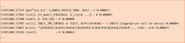 Figure 2F: Strace Excerpt of F90 One-by-One Code: 256 Iterations
In fact, I did get a 6,144-byte write that finished in 0.000027 seconds, which is a throughput of 227.5GBps. The speed is well above the speed of the single disk used in these runs, so I know there are some caching effects. (Caching effects probably show up in all the examples in this series because the I/O is so small; however, my focus is not really on the throughput itself, but on the I/O pattern.)
The strace output in Figure 3F is for 500 iterations.
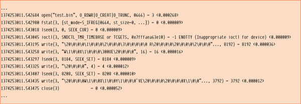 Figure 3F: Strace Excerpt of F90 One-by-One Code: 500 Iterations
The 500-iteration example shows four writes interspersed with lseeks. The largest write is 8,192 bytes, the buffer size limit, followed by smaller writes. This write pattern is a result of how the code writes and how the library handles the extra 4 bytes before and after the record.
The strace output for the 2,000-iteration example is shown in Figure 4F.
 Figure 4F: Strace Excerpt with F90 One-by-One Code with 2,000 Iterations
Notice the considerable number of writes (16) coupled with a number of lseeks. Also notice that some of the writes do not represent a fully filled buffer. Again, this is because of the way Fortran (the GFortran compiler in particular) writes unformatted data. To some people, this will look like an IOPS-driven application with a number of lseeks, which can hurt performance; however, as was the case with the C code, I am relying on the OS to combine writes and then perform them as a single streaming write.
Just as with the C code, I might have better ways to do output with the Fortran code. To begin, I’ll try performing the same steps I used with the C code by creating an array of the user-defined data type and then writing the entire array to a file with a single write statement (Listing 2F). To run this code for a different number of data elements, I need to change lines 12 and 14. To make life easier, I will refer to this as the “array” code, as I did with the C example.
Listing 2F: F90 Code Example with Output in Loop (Array)
 1    program ex1a
 2
 3    type rec
 4       integer :: x, y, z
 5       real :: value
 6    end type rec
 7
 8    integer :: counter
 9    integer :: counter_limit
10    integer :: ierr
11
12    type (rec) :: my_record(2000)
13
14    counter_limit = 2000
15
16    ierr = -1
17    open(unit=8, file="test.bin", status="replace", &
18         action="readwrite", form="unformatted", &
19         iostat=ierr)
20    if (ierr > 0) then
21       write(*,*) "error in opening file! Stopping"
22       stop
23    else
24       do 10 counter=1,counter_limit
25          my_record(counter)%x = counter
26          my_record(counter)%y = counter + 1
27          my_record(counter)%z = counter + 2
28          my_record(counter)%value = counter * 10.0
29 10    continue
30    endif
31    write(8) my_record
32    close(8)
33
34    end program ex1a
35
First, I’ll try 100 elements to see if anything weird is happening in the strace output (Figure 5F).
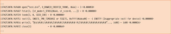 Figure 5F: Strace Excerpt of F90 Array Code: 100 Elements
The strace output looks almost identical to the strace output from the previous Fortran code. However, the amount of data is different – 1,608 bytes instead of 2,400 bytes – because I’m writing 100 elements as a continuous record, or 16 bytes x 100 elements = 1,600 bytes. Remember, though, that unformatted data records in GFortran, and almost all Fortran standards, have an additional 4 bytes at the beginning and end of the record, making a total of 1,608 bytes.
Similarly, a 256-element run (Figure 6F) and a 500-element run (Figure 7F) would have write() functions of 4,096 and 8,000 bytes of data (16 bytes x 256 elements and 16 bytes x 500 elements), respectively. The extra 4 bytes at the beginning and end of the record make 4,104 bytes for the 256-element example and 8,008 bytes for the 500-element example, which match the corresponding strace output snippets.
 Figure 6F: Strace Excerpt of F90 Array Code: 256 Elements
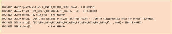 Figure 7F: Strace Excerpt of F90 Array Code: 500 Elements
The 500-element strace in Figure 7F only has one write() function call, whereas the one-by-one version of the code (Figure 3F) has four writes with lseeks in between. Because the array code has just 8,008 bytes of data, which is smaller than the buffer size (8,192 bytes), the data can be output with a single call to write().
Finally, the 2,000-iteration example (Figure 8F) shows five writes instead of the 16 needed for the one-by-one code (Figure 4F), as well as just one lseek, as opposed to a number of them in the one-by-one code. The first three writes in this last example use the maximum buffer size (8,192 bytes), then finishes outputting the data with a 7,432-byte write, and ends with a final write for the last 4 bytes at the end of the record.
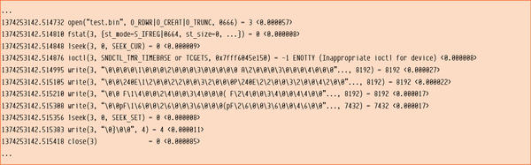 Figure 8F: Strace Excerpt of F90 Array Code: 2,000 Elements
If you compare this strace output with that in Figure 8C of the previous article, which is from the C code that uses a buffer, you will see that the C code exceeded the buffer size, reaching 28,672 bytes in the first write. However, Fortran I/O is always limited to 8,192 bytes per write() function, which means the Fortran code relies much more heavily on the OS than does the C code to combine writes for better throughput performance.
Summary
As the Fortran examples show here, you can get a great deal of useful information from strace output that you can use to help in understanding the I/O patterns of an application The C examples of the previous article in the series showed how you could improve throughput performance by sequentially streaming an I/O pattern to the OS. This kind of input also helps the OS because it can tell the file system to open a file with a large number of allocated blocks, hopefully sequential, to which data can then be streamed to the underlying storage media, which is what hard drives really like.
The same isn’t always true for Fortran. Fortran, and more specifically GFortran, is limited to I/O buffers of 8,192 bytes. Fortran therefore has to rely on the underlying OS to combine writes. GFortran also likes to intersperse lseeks between writes, which can also reduce throughput. For better I/O performance in Fortran, then, you might be better off using a library or abstraction for I/O, such as hdf5, or even writing your own C library that you can link to your Fortran code.
In the final article of this series, I look at I/O patterns in Python programs.