
In the last of this four-part series on using Warewulf to build an HPC cluster, I focus a bit more on the administration of a Warewulf cluster, particularly some basic monitoring and the all-important resource manager.
Warewulf Cluster Manager – Part 4
In this series on using Warewulf to build an HPC cluster, the first focus was on getting the master node to deploy compute nodes easily and then adding some tools to make the cluster useful (NFS mounts from the master node, user accounts on all of the nodes – recall that the nodes are separate from one another so user accounts aren't on the compute nodes unless you put them there, a parallel shell that allows you to run commands easily on a range of nodes, and NTP on the cluster so the clocks are synchronized). Next, attention was turned to the user by creating and configuring the development and run-time environments and adding Environment Modules, which allow you to control the choice of development tools you use to build and run applications on your cluster. In this final article, I turn my attention back to administration, primarily toward some basic monitoring tools and installation of the final piece of the cluster – the resource manager.
One would think that building an HPC cluster would just be a simple matter of slapping some boxes together with a network and calling it a day. This might work with flashmob computing, but if you've followed this series, you realize this is not the usual case. If you want to put together an HPC cluster that has the tools for building and running applications, can be scaled (i.e., nodes can be added or removed easily), and has administration tools and tools for users who want to use the cluster, then you really have to pay attention to the design of the cluster and the software. This doesn't mean it has to be difficult, but you just have to learn how to think a bit differently.
The first step in thinking differently is to realize that a cluster is a group of disparate systems. Each one has its own OS. Understanding this concept means that you now realize that you have to use tools to make sure the OS on the various nodes is the same (or really close) and that the administrator can easily update the OS and put it on the compute nodes within the cluster. Warewulf provides much of this functionality, with the side benefit of being stateless (i.e. no disk required), which means that when the compute nodes are rebooted they get the current OS image. In the case of Warewulf, it also means that the image is so small it can be transferred to the compute nodes and installed quickly and take up very little memory. Because Warewulf is stateless, if the node needs to update the OS, you just power-cycle the node(s) and a new image is transferred. Otherwise, you have to worry about what bits and pieces of the OS are on which node, and you can end up with what is referred to as OS skew, in which no two nodes are exactly the same.
However, having a tool that allows you to send an OS to the compute nodes does not a real working cluster make. This is true even if you are putting together two systems to learn about HPC or if you are building the largest system in the world. What makes a cluster easy to use and manage are the additional tools that are layered on top of this basic functionality. When selecting and installing these tools you have to keep reminding yourself that the nodes are distinct. You need to select tools that make life easier for both the user and the administrator and that are easy to integrate into the cluster deployment tool (in this case, Warewulf).
In this article, I add some monitoring and management tools to the cluster that can make your life with an HPC cluster a bit easier. The first two tools, GKrellM and Ganglia, allow you to monitor what is happening on your cluster. These types of tools are really indispensable when you want to run an HPC cluster, even if just to run your applications.
The final piece I’m going to add is a resource manager, also commonly called a job scheduler. It allows users, or even administrators, to create and send a script that runs their application to a scheduler that executes the script when the resources are available. Although strictly speaking, you don't need this tool because you can run jobs by specifying which user can run on which nodes, this tool makes your life much, much easier. You can submit “jobs” to the resource manager and then walk away from your desk and do something else. Coupling a resource manager with Environment Modules allows you to run applications more easily that have different environment requirements, such as different MPI libraries.
For this article, as with the previous ones, I will use the exact same system. The purpose of this article is not to show you how to build various toolkits for the best performance or how to install packages on Linux. Rather, I’m using these toolkits as examples of how to build your HPC development and run-time environment with Warewulf. At the same time, I'm choosing toolkits that are very commonly used in HPC, so I'm not working with something obscure; these toolkits have been proven to be useful in HPC. I’m also choosing to build the toolkits from source rather than install them from an RPM (where possible). This allows me to have control over where they are installed and how they are built.
Cluster Monitoring
The first toolkit I want to discuss allows you to monitor the nodes in your cluster. In this case, monitor means watching the load on the node – basically the same as running top or uptime on each node. This information is very useful to an administrator because it can tell which nodes are being used, how much they are being used, what the network load is on the nodes, and so on. In essence, it’s a snapshot of how the cluster is performing. Administrators will use these tools to determine whether any nodes are down (i.e., not responding) and the utilization of the cluster (i.e., which nodes are idle and not being used).
In this section of the article, I’m going to discuss three different ways to monitoring your cluster, starting with something really simple that gives you an idea which nodes are down and which ones are idle.
Simple Option – pdsh and uptime
In part 2, Installing and Configuring Cluster Tools, pdsh was installed on the master node so you could run the same command on a range of nodes. Therefore, you can use pdsh with other commands to query the list of nodes and gather information on the status of the nodes. For example, it’s pretty easy to run uptime on all of the nodes in the cluster (currently, I have just two nodes: test1, which is the master node, and n0001, which is the first compute node):
[laytonjb@test1 ~]$ pdsh -w test1,n0001 uptime
test1:  18:57:17 up  2:40,  5 users,  load average: 0.00, 0.00, 0.02
n0001:  18:58:49 up  1:13,  0 users,  load average: 0.00, 0.00, 0.00
With a simple Bash, Perl, or Python script and pdsh, you can query almost anything. Just be warned that you need to play “defense” with your scripts to filter out nodes that are down. For example, if I shut off node n0001, then the same command I used above looks like this:
[laytonjb@test1 ~]$ pdsh -w test1,n0001 uptime
test1:  18:59:43 up  2:42,  5 users,  load average: 0.05, 0.02, 0.01
n0001: ssh: connect to host n0001 port 22: Connection timed out
pdsh@test1: n0001: ssh exited with exit code 255
You can do many other things with pdsh. For example, you can use it inside some sophisticated scripts to collect data from nodes. You can put these scripts in a cron job and gather the results in something like a “health database” that holds status and “health” information about the cluster. You can even get creative and plot the data to a web interface for the admin and users to view. It’s also very useful if you need to produce reports that help justify the purchase of hardware. Needless to say, this simple approach to monitoring could be used in many ways. As an example of what you can do with simple scripting, one of the first tools I ever used in clusters is called bWatch, which simply takes data from something like pdsh and creates a graphical table using TCL/TK.
In some cases, however, you might want graphical output, so you can get an immediate picture as to the status of the cluster (“status at a glance”). In the next two sections, I present two options for graphical monitoring of clusters.
Cluster Monitoring for Smaller Systems – GKrellM
For smaller systems, you could use GKrellM, either in place of pdsh or to supplement it. Gkrellm is a simple tool that gathers information about your system and displays it in a small application. It is fairly common for desktops and has a nice stacked set of charts and information that people put on the one side of their screen or the other, as in Figure 1.

Figure 1: GKrellM Example from gkrellm.net
You can see in the figure that GKrellM is monitoring many aspects of the system. Starting at the top and working down the image, you see the kernel version, uptime, current CPU load on all processors (four, in this case), temperatures and fan speeds (from lm-sensors), total disk usage and the usage of each disk, network usage, and memory usage including swap. All of this information is configurable, including the theme or the appearance.
One cool thing about GKrellM is that you can install a daemon version of it on compute nodes and then display the data on you desktop in a different GKrellM window. Here, I'll explain how you can use the daemon for monitoring smaller clusters, which is quite simple, with Warewulf. The output (Listing 1) of my install of gkrellmd, the daemon, into the VNFS shows that it is very small.
To make sure gkrellmd starts when the node boots, I’ll modify the /etc/rc.d/rc.local file slightly (don't forget its location is really /var/chroots/sl6.2/etc/rc.d/rc.local):
[root@test1 rc.d]# more rc.local
#!/bin/sh
#
# This script will be executed *after* all the other init scripts.
# You can put your own initialization stuff in here if you don't
# want to do the full Sys V style init stuff.

touch /var/lock/subsys/local

/sbin/chkconfig iptables off
/sbin/service iptables stop
/sbin/chkconfig ntpd on
/sbin/service ntpd start
/sbin/service gkrellmd restart
All I did was make sure the GKrellM daemon was started when the node booted.
I also need to edit the /var/chroots/sl6.2/etc/grkellmd.conf GKrellM configuration file in the VNFS by appending the following lines to the file:
update-hz 3
port 19150
allow-host      10.1.0.250
fs-interval 2
nfs-interval 16
inet-interval 0
Then, on the master node (i.e., IP address 10.1.0.250 above), I need to create a GKrellM user:
[root@test1 ~]# useradd -s /bin/false gkrellmd
Because I made changes to the VNFS, the final step is to rebuild the VNFS with the wwvnfs command:
[root@test1 ~]# wwvnfs --chroot /var/chroots/sl6.2  --hybridpath=/vnfs
Using 'sl6.2' as the VNFS name
Creating VNFS image for sl6.2
Building template VNFS image
Excluding files from VNFS
Building and compressing the final image
Cleaning temporary files
WARNING:  Do you wish to overwrite 'sl6.2' in the Warewulf data store?
Yes/No> y
Done.
[root@test1 ~]# wwsh vnfs list
VNFS NAME                 SIZE (M)
sl6.2                     71.4
The VNFS is only 71.4MB after adding the gkrellmd RPM. The size of the VNFS directly affects the amount of data that needs to be sent to the compute nodes, and 71.4MB is really quite small in this case.
After booting the compute node, I can run the following command as a user to see the gkrellm for the compute node.
[laytonjb@test1 ~]$ gkrellm -s n0001&
Notice that I put the command in the background using the & character at the end of the command. This means I won’t tie up a terminal window running gkrellm for that compute node. The gkrellm for the compute node should immediately pop up on the screen (Figure 2).
 Figure 2: Gkrellm on the master node showing the status of both nodes (master and first compute).
In case you are curious, the first compute node does have three cores (it’s an AMD node).
You can run gkrellm as a user or an administrator, which is nice for scenarios when perhaps you have the cluster to yourself or you have a small cluster that only you use. It’s also nice for small clusters in general. However, if you have a larger number of nodes, you will fill up the window with the gkrellms for each compute node. For larger clusters, you can use another common cluster monitoring tool – ganglia.
Cluster Monitoring for Larger Systems – Ganglia
Ganglia is a monitoring system designed for distributed systems and is designed to be scalable to a fairly large number of nodes (think thousands). It is very customizable, allowing you to develop monitoring metrics on your own and to change aspects, such as the frequency at which data is reported and the units for different metrics. You also have many ways to display the data, with the primary choice being web based.
Installing and getting ganglia to function is fairly straightforward. I downloaded the latest RPMs from the ganglia website (they are typically built for RHEL, so CentOS or Scientific Linux works almost every time). On the master node, I first installed the ganglia library (Listing 2). Notice that Yum pulled in several dependencies for me. Moreover, notice that the size of the packages are all pretty small. In addition to monitoring the compute nodes, I also like to monitor the master node; therefore, the next RPM to install is the monitoring daemon gmond (Listing 3).
The next RPM to install into the master node is the data collection tool called ganglia-metad. This set of tools gathers data from the various ganglia monitoring daemons (gmond) and collects them (Listing 4). This installation pulls in a fair number of dependencies, but I don't mind too much because it’s the master node, has plenty of disk space, and only has to be installed once.
The final RPM to be installed on the master node is the web interface for ganglia (Listing 5). The installation installed some PHP tools, which means the ganglia web interface is PHP based.
All the necessary components of ganglia are installed on the master node: the ganglia base (libganglia), the monitoring daemon (gmond), the data collection tools (gmetad), and the web interface. The next step is to get it running on the master node, which is pretty easy but requires a few steps. The first task is to make sure, with the use of chkconfig, that ganglia always starts when the master node boots:
[root@test1 ganglia]# chkconfig --list | more
NetworkManager  0:off   1:off   2:on    3:on    4:on    5:on    6:off
acpid           0:off   1:off   2:on    3:on    4:on    5:on    6:off
atd             0:off   1:off   2:off   3:on    4:on    5:on    6:off
auditd          0:off   1:off   2:on    3:on    4:on    5:on    6:off
autofs          0:off   1:off   2:off   3:on    4:on    5:on    6:off
avahi-daemon    0:off   1:off   2:off   3:on    4:on    5:on    6:off
certmonger      0:off   1:off   2:off   3:off   4:off   5:off   6:off
cgconfig        0:off   1:off   2:off   3:off   4:off   5:off   6:off
cgred           0:off   1:off   2:off   3:off   4:off   5:off   6:off
conman          0:off   1:off   2:off   3:off   4:off   5:off   6:off
cpuspeed        0:off   1:on    2:on    3:on    4:on    5:on    6:off
crond           0:off   1:off   2:on    3:on    4:on    5:on    6:off
cups            0:off   1:off   2:off   3:off   4:off   5:off   6:off
dhcpd           0:off   1:off   2:on    3:on    4:on    5:on    6:off
dhcpd6          0:off   1:off   2:off   3:off   4:off   5:off   6:off
dhcrelay        0:off   1:off   2:off   3:off   4:off   5:off   6:off
dnsmasq         0:off   1:off   2:off   3:off   4:off   5:off   6:off
gmetad          0:off   1:off   2:on    3:on    4:on    5:on    6:off
gmond           0:off   1:off   2:on    3:on    4:on    5:on    6:off
haldaemon       0:off   1:off   2:off   3:on    4:on    5:on    6:off
...
Then, I need to restart PHP and HTTPd with the service php restart and service httpd restart commands then start gmond and gmetad with service:
[root@test1 ~]# service gmond start
Starting GANGLIA gmond:                                    [  OK  ]
[root@test1 ~]#
[root@test1 ~]# service gmetad start
Starting GANGLIA gmetad:                                   [  OK  ]
Now everything should just work. To find out, go to http://localhost/ganglia (localhost is the name of the master node as far as Apache is concerned). This page should look something like Figure 3.
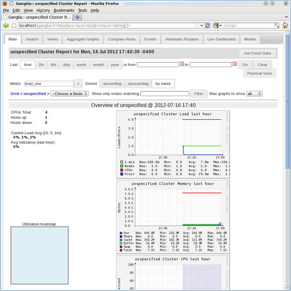 Figure 3: Ganglia web page output for the master node only.
You can tell that this only covers the master node because the compute nodes should not be booted (yet) and the web page shows only one host (look for the phrase Hosts up), which is the master node.
The next step is to install ganglia into the VNFS. I really only need the monitoring daemon, gmond, but that means I need libganglia as well. Rather than list the output from Yum, I’ll just list the two commands needed to install the RPMs into the VNFS:
yum --tolerant --installroot /var/chroots/sl6.2 -y install libganglia-3.4.0-1.el6.i686.rpm
yum --tolerant --installroot /var/chroots/sl6.2 -y install ganglia-gmond-3.4.0-1.el6.i686.rpm
Recall that /var/chroots/sl6.2 is the path to the VNFS on the master node here, but I’m not quite done yet.
By default, ganglia uses multicast to allow all of the nodes to broadcast their data to the master node (the gmetad). However, not all network switches – particularly for small home systems – can handle multicast. As suggested by a person on the Ganglia mailing list, I changed ganglia to use unicast. The changes are pretty easy to make.
The primary file to edit is gmond.conf, which is on both the master node and the compute nodes (VNFS). For the VNFS, the full path is /var/chroots/sl6.2/etc/ganglia/gmond.conf. For the master node, the full path is /etc/ganglia/gmond.conf. I have to change two sections of the file on both the master node and the compute node as follows:
udp_send_channel {
  host = 10.1.0.250
  port = 9649
}

udp_recv_channel {
  port = 9649
}
Before these changes are made, the udp_send_channel function will probably have the mcast_join term, which means it was set up for multicast. The changes above, which are done on both the master node and the VNFS, will switch it to unicast (be sure to erase the line with mcast_join).
One last suggestion is to give the option send_metadata_interval a larger number in the VNFS gmond.conf file. This is the number of seconds between which the data is sent to the metadata server (gmetad), which is the master node. I switched it to 15 to help control the flow of traffic to the master node from the compute nodes.
After adding the RPMs and editing the files, you have to rebuild the VNFS with the command
wwvnfs --chroot /var/chroots/sl6.2 --hybridpath=/vnfs
The VNFS grew a little bit in size from the ganglia additions to 72.3MB, which is still pretty small.
Now I can boot the compute node. Once it comes up (check this by sshing to the node as a user – if it works, the node is “up”) I can open a web page with the URL http://localhost/ganglia. Figure 4 is a screenshot after I chose to go to the first compute node (n0001).
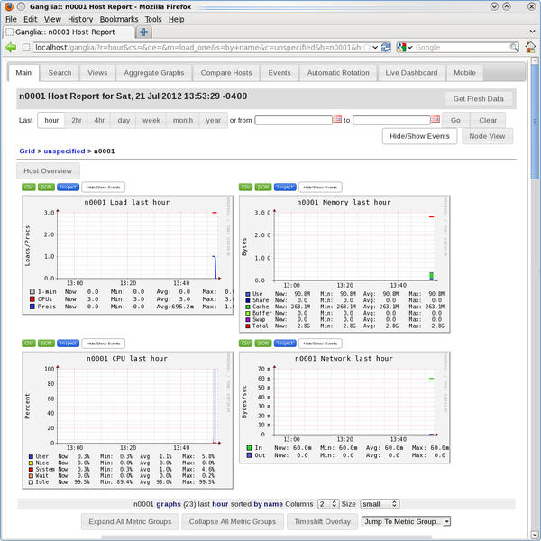 Figure 4: Ganglia web page including first compute node
I had just started the first compute node, so very little information is there, but the mere fact that there is an image indicates success.
Cluster Resource Management
From the very beginning of HPC, people have had to share systems. One technique to do so was generically called “resource management.” The more common phrase is “job scheduler.” The idea is simple – users write small scripts, commonly called “jobs,” that define what they want to run and submit it to a resource manager. The manager then examines the job file and makes a list of the needed resources (how many nodes, how much time, etc.), and when the resources are available, the resource manager executes the job script on behalf of the user. Typically this approach is for batch jobs – jobs that are not interactive. However, it can also work for interactive jobs for which the resource manager gives you a prompt to the node that is running your “job,” which is really just a shell. Then, you can run whatever application you want from that point on.
You have several options for resource managers. Some are commercially supported and some are open source, either with or without a support option. I will use Torque, which is a development of the old PBS (Portable Batch System) resource manager. Torque has come a long way since the old PBS days and is supported by Adpative Computing if you want support. I will be using version 4.0.2, which I downloaded from the Torque site. As a quick note, even though it is called Torque, you will see “PBS” or “pbs” used to refer to details of the application. Don’t be confused – the application is Torque.
Before talking about how to build and install Torque, I’ll talk about the basic architecture and what I’m going to install on the compute nodes. Torque has three basic parts: (1) The server (pbs_server), (2) the scheduler (pbs_sched), and (3) the worker, which is called “mom” or pbs_mom. The server is the piece that accepts the jobs, and the scheduler determines what to run on what compute nodes. The pbs_mom communicates back to the core parts (pbs_server and pbs_sched), telling Torque the status of the compute nodes, such as what they are running or whether they are free to execute applications.
Typically, in clusters, the server and the scheduler will be run on the master node. Then you run the mom on the worker node(s) or wherever you want to run jobs. In this case, I’ll run it on the compute node(s). Translating this to RPMs, pbs_server and pbs_sched will be installed on the master node and pbs_mom will be installed on the compute node(s). More specifically, I will install the server and the scheduler in /opt/torque so it is accessible by all nodes (not necessary, but useful). Then, I will install pbs_mom into the VNFS, but I will point pbs_mom to put the logs in /opt/torque/mom_logs because it's not really an effective use of memory to store logs for Torque (remember that Warewulf uses memory for the base distribution). The pbs_mom element does not take up a lot of space, so I'm not too concerned about installing it in the VNFS.
This split in installation – the server and scheduler in /opt/torque and pbs_mom in /usr – will require the Torque RPMs to be built twice, but this is really not a difficult or time-consuming process. The maintainer of the RPM spec file for Torque, Michael Jennings, gave me some tips to save time when using the Torque source file (the .tar.gz file). The RPM spec file is included in the source, so you can use the command rpmbuild to built the various Troque RPMs.
The first step is to build the RPMs for the server and scheduler, which are being installed on the master node. The command to build from the .tar.gz file is:
rpmbuild --define '_prefix /opt/torque'
         --define '_includedir /opt/torque/include'
         --define 'torque_home /opt/torque' -ta torque-4.0.2.tar.gz
You have to run this command as root. Notice that the build variables prefix, includedir, and torque_home are defined as /opt/torque. The rpmbuild command created a directory, /root/rpmbuild/RPMS/x86_64, in which the RPMs are located. I installed the torque RPM, the torque-server RPM, and the torque-scheduler RPM (note that this is a simple first-in, first-out [FIFO] scheduler). The install commands are:
[root@test1 x86_64]# yum install ./torque-4.0.2-1.cri.x86_64.rpm
...
[root@test1 x86_64]# yum install ./torque-scheduler-4.0.2-1.cri.x86_64.rpm
...
[root@test1 x86_64]# yum install ./torque-server-4.0.2-1.cri.x86_64.rpm
I didn’t show the output from Yum for each of the installations because there were no dependencies when the RPMs were installed in this order.
A slight bug shows up during the installation of Torque 4.0.2. After everything is installed, you need to create a directory named /opt/torque/checkpoint on the master node. Without it, the next steps will fail.
After you create this directory, you can then create the definitions for the Torque server on the master node. You run the command pbserver -t create. After the server has been created, you can see the server definitions using the following command:
[root@test1 ~]# qmgr -c 'p s'
#
# Set server attributes.
#
set server acl_hosts = test1
set server log_events = 511
set server mail_from = adm
set server scheduler_iteration = 600
set server node_check_rate = 150
set server tcp_timeout = 300
set server job_stat_rate = 45
set server poll_jobs = True
set server mom_job_sync = True
set server next_job_number = 0
set server moab_array_compatible = True
This is the basic server definition, but it is still missing some details for a queue, or the “holding” place for jobs that have been submitted. Multiple queues can be defined by the administrator. For the purpose of this article, I’m just going to define what is called a simple “batch” queue. That is, a queue that schedules and then runs jobs submitted in batch mode. This queue is not difficult to create with the qmgr (queue manager) command:
qmgr -c "set server scheduling=true"
qmgr -c "create queue batch queue_type=execution"
qmgr -c "set queue batch started=true"
qmgr -c "set queue batch enabled=true"
qmgr -c "set queue batch resources_default.nodes=1"
qmgr -c "set queue batch resources_default.walltime=3600"
qmgr -c "set server default_queue=batch"
I also modified two settings to the server:
[root@test1 ~]# qmgr -c "set server operators += laytonjb@test1"
[root@test1 ~]# qmgr -c "set server managers += laytonjb@test1"
[root@test1 ~]# qmgr -c "set server operators += root@test1"
[root@test1 ~]# qmgr -c "set server managers += root@test1"
Running the qmgr command again gets details on the server and queue definitions.
[root@test1 ~]# qmgr -c 'p s'
#
# Create queues and set their attributes.
#
#
# Create and define queue batch
#
create queue batch
set queue batch queue_type = Execution
set queue batch resources_default.nodes = 1
set queue batch resources_default.walltime = 01:00:00
set queue batch enabled = True
set queue batch started = True
#
# Set server attributes.
#
set server scheduling = True
set server acl_hosts = test1
set server managers = laytonjb@test1
set server operators = laytonjb@test1
set server default_queue = batch
set server log_events = 511
set server mail_from = adm
set server scheduler_iteration = 600
set server node_check_rate = 150
set server tcp_timeout = 300
set server job_stat_rate = 45
set server poll_jobs = True
set server mom_job_sync = True
set server next_job_number = 0
set server moab_array_compatible = True
One last thing you need to do is tell the server the name of the nodes it can use and how many cores it has. To do this, you edit a file /opt/torque/server_priv/nodes as root. In the example here, the file should look like this:
n0001 np=3
You should read the manual for information on the np option, but really quickly, I like to run on all of the processors on the nodes. No fewer or no more than the node has. For my cluster, the master node, test1, has four real cores. The compute node is an older system that has three real cores (np=3). Yes, there are systems that have only three cores.
I also should check the server configuration quickly to make sure it is working. The first command, qstat, checks the status of the queues:
[laytonjb@test1 ~]$ qstat -q

server: test1

Queue            Memory CPU Time Walltime Node  Run Que Lm  State
---------------- ------ -------- -------- ----  --- --- --  -----
batch              --      --       --      --    0   0 --   E R
                                               ----- -----
                                                   0     0
This is the expected output (please check the Torque manual for more details).
A second command, pbsnodes, can be used to find out which nodes in the cluster have been defined and which ones are up (available for running applications) or down (not available):
[laytonjb@test1 ~]$ pbsnodes -a
test1
     state = down
     np = 1
     ntype = cluster
     mom_service_port = 15002
     mom_manager_port = 15003
     gpus = 0
n0001
     state = down
     np = 3
     ntype = cluster
     mom_service_port = 15002
     mom_manager_port = 15003
     gpus = 0
By default, Torque defines the first node as the master node, even though I have not installed pbs_mom on the master node. The output is as expected (please check the Torque manual for more details).
The next step is to rebuild the Torque RPMs for the compute node and install them into the VNFS. Rebuilding them is pretty simple. In the directory where the Torque source .tar.gz file is located, you just run the command
rpmbuild -ta torque-4.0.2.tar.gz
This creates all of the Torque RPMs in the directory /root/rpmbuild/RPMS/x86_64. It also overwrites the previous RPMs that were used for the master node, so you might want to copy those to a new subdirectory before creating the new ones.
Once the new RPMs are created, just use the yum command to install them into the VNFS:
[root@test1 x86_64]# yum --tolerant --installroot /var/chroots/sl6.2 -y install
[root@test1 x86_64]# yum --tolerant --installroot /var/chroots/sl6.2 -y install torque-client-4.0.2-1.cri.x86_64.rpm
The next step is to install the Torque pbs_mom into the VNFS. By default, Torque will put its logs in /var/spool/torque/mom_logs, which uses memory in Warewulf – a somewhat undesirable situation. Up to this point, Warewulf has provided a great number of advantages, but storing Torque logs on the compute nodes is perhaps a waste. It is better to store them on the master node in an NFS directory. Fortunately this is simple to do. In the VNFS, create the file /etc/sysconfig/pbs_mom. For the VNFS, the full path is /var/chroots/sl6.2/etc/sysconfig/pbs_mom. The file entries should look like the following:
[root@test1 sl6.2]# more etc/sysconfig/pbs_mom

PBS_LOGFILE=/opt/torque/mom_logs/`hostname`.log
export PBS_LOGFILE

args="-L $PBS_LOGFILE"
The pbs_mom script automatically looks for this file on startup and will define the location or the pbs_mom logs as /opt/torque/mom_log (it’s an NFS-served directory). For the first compute node, n0001, the logfile will be called n0001.log.
Watch out for a few gotchas when writing logs to the NFS server. Some of these problems occur because, by default, SL 6.2 uses NFSv4. Fewer problems would be encountered if the compute nodes mounted the NFS filesystem as NFSv3. Although it sounds a bit strange, it can solve lots of problems and is fairly easy to do by editing the file /var/chroots/sl6.2/etc/fstab so that the NFS mounts use NFSv3:
[root@test1 etc]# more fstab
#GENERATED_ENTRIES#
tmpfs /dev/shm tmpfs defaults 0 0
devpts /dev/pts devpts gid=5,mode=620 0 0
sysfs /sys sysfs defaults 0 0
proc /proc proc defaults 0 0
10.1.0.250:/var/chroots/sl6.2 /vnfs nfs nfsvers=3,defaults 0 0
10.1.0.250:/home /home nfs nfsvers=3,defaults 0 0
10.1.0.250:/opt /opt nfs nfsvers=3,defaults 0 0
10.1.0.250:/usr/local /usr/local nfs nfsvers=3,defaults 0 0
Notice the addition of the option nfsvers=3.
The Torque installation in the VNFS also needs a couple of quick modifications. The first is to define the Torque server by editing the /var/chroots/sl6.2/var/spool/torque/server_name file:
test1
The second modification is to edit the /var/chroots/sl6.2/var/spool/torque/mom_priv/config file:
$pbsserver test1$logevent 225
At this point, you just need to rebuild the VNFS and boot some compute nodes. To do this, use the wwvnfs command:
[root@test1 x86_64]# wwvnfs --chroot /var/chroots/sl6.2  --hybridpath=/vnfs
Using 'sl6.2' as the VNFS name
Creating VNFS image for sl6.2
Building template VNFS image
Excluding files from VNFS
Building and compressing the final image
Cleaning temporary files
WARNING:  Do you wish to overwrite 'sl6.2' in the Warewulf data store?
Yes/No> y
Done.
[root@test1 sysconfig]# wwsh vnfs list
VNFS NAME                 SIZE (M)
sl6.2                     74.3
The VNFS at the beginning was 55.3MB in size, so the size of the VNFS itself has increased by about 50%. This might sound like quite a bit, but when you consider that even home systems have 2-4GB of memory, this is not much space. Plus, you have gained quite a bit of functionality.
In case you are interested, after booting the first compute node, I did a df to see how much space was used:
bash-4.1# df -h
Filesystem            Size  Used Avail Use% Mounted on
none                  1.5G  274M  1.2G  19% /
tmpfs                 1.5G     0  1.5G   0% /dev/shm
10.1.0.250:/var/chroots/sl6.2
                       53G   33G   18G  66% /vnfs
10.1.0.250:/home       53G   33G   18G  66% /home
10.1.0.250:/opt        53G   33G   18G  66% /opt
10.1.0.250:/usr/local
                       53G   33G   18G  66% /vnfs/usr/local
The installed distro uses about 274MB of memory, which is not bad considering the benefits of using Warewulf!
One last thing to check before submitting a job is whether the Torque server can communicate with the compute node:
[root@test1 ~]# pbsnodes -a
n0001
     state = free
     np = 3
     ntype = cluster
     status = rectime=1343594239,varattr=,jobs=,state=free,netload=118255091,gres=,loadave=0.02,ncpus=3,physmem=2956668kb,availmem=2833120kb,totmem=2956668kb,idletime=107,nusers=0,nsessions=0,uname=Linux n0001 2.6.32-220.el6.x86_64 #1 SMP Sat Dec 10 17:04:11 CST 2011 x86_64,opsys=linux
     mom_service_port = 15002
     mom_manager_port = 15003
     gpus = 0

test1
     state = down
     np = 4
     ntype = cluster
     mom_service_port = 15002
     mom_manager_port = 15003
     gpus = 0
You can easily see that the Torque server can communicate with the first compute node, and it is ready to go with three processors (np=3).
Final Exam
The cluster still needs to take a final exam to make sure it is working correctly. For this final exam, I’ll run an MPI application on the compute node that has three cores, and for extra credit, I’ll use the Open64 compilers and MPICH2, so I have to use modules.
The program I’ll be using is a simple MPI code for computing pi (3.14159…). The code is a Fortran90 example. Building the code is very easy using Environment Modules:
[laytonjb@test1 TEST]$ module load compilers/open64/5.0
[laytonjb@test1 TEST]$ module load mpi/mpich2/1.5b1-open64-5.0
[laytonjb@test1 TEST]$ module list
Currently Loaded Modulefiles:
  1) compilers/open64/5.0         2) mpi/openmpi/1.6-open64-5.0
[laytonjb@test1 TEST]$ mpif90 mpi_pi.f90 -o mpi_pi
Next you need to write a Torque job script. This is a simple Bash script, but it is very easy to get carried away and write a complicated script. I found a script at the University of Houston Research Center that I used as a starting point. It is well commented and has some nice things already in the sample script. The final Torque job script I used is in Listing 6.
The script has line numbers to make a discussion much easier. Any directive to Torque starts with #PBS, such as line 12. Therefore, comments begin with ###, such as line 2. Lines 22-24 load the Environment Modules the application needs. The script writes out some simple information in lines 38-41, that can be very helpful. Finally, the application executes in line 43. The input to the application is file1. Now I’m ready to submit the job script to Torque:
[laytonjb@test1 TEST]$ qsub pbs-test_001
19.test1
[laytonjb@test1 TEST]$ qstat -a

test1:
                                                                         Req'd  Req'd   Elap
Job ID               Username    Queue    Jobname          SessID NDS   TSK    Memory Time  S Time
-------------------- ----------- -------- ---------------- ------ ----- ------ ------ ----- - -----
10.test1             laytonjb    batch    mpi_pi_fortran90    --      1      3    --  00:10 Q   --
The qstat command gets the status of the queues in Torque, and the -a option tells it to check all queues.
Once the job is finished, you will see two files in the directory in which it ran: pbs-test_001.e19 and pbs-test_001.o19. The first file contains any stderr messages, and the second contains the output from the job script (all of the extra information in the job script):
[laytonjb@test1 TEST]$ more mpi_pi_fortran90.o19
Working directory is /home/laytonjb/TEST
Running on host n0001
Start Time is Tue Aug  7 19:00:00 EDT 2012
Directory is /home/laytonjb/TEST
Using 3 processors across 1 nodes
End time is Tue Aug  7 19:00:01 EDT 2012
The output from the application is in output.mpi_pi:
[laytonjb@test1 TEST]$ more output.mpi_pi
 Enter the number of intervals: (0 quits)
 pi is  3.1508492098656031  Error is 9.25655627581001283E-3
I think the cluster has passed the final exam.
Final Words – Preconfigured Warewulf
This is the fourth and final article in the Warewulf series. Warewulf is a very powerful and flexible cluster toolkit, and in my mind, it is also fairly easy to use. However, some people might balk at the work involved and look for something simpler but that also has the features of Warewulf. The solution for this is Basement Supercomputing.
Basement Supercomputing has taken all of the steps and details of installing and configuring Warewulf and the extra tools and put them into a very neat package. They are doing this as part of their Limulus project, which is developing a small cluster that fits into a standard ATX-type case.
I admit that I got stuck at several points in this series, and Douglas Eadline at Basement Supercomputing helped me get past them. Their prebuilt Warewulf stack is really nice and amazingly easy to use. It has virtually all of the tools mentioned in this series, although right now, they are using SGE (Sun Grid Engine) as a resource manager. They also have a few open source tools that can help you monitor and manage your cluster.