
You have parallelized your serial application, but as you use more cores you are not seeing any improvement in performance. What gives?
Why Good Applications Don’t Scale
You just bought a new system with lots and lots of cores (e.g., a desktop with 64 cores or a server with 128 cores). Now that you have all of these cores, why not take advantage of them by parallelizing your code? Depending on your code and your skills, you have a number of paths to parallelization, but after some hard work profiling and lots of testing, your application is successfully parallelized – and it gives you the correct answers! Now comes the real proof: You start checking your application’s performance as you add processors.
Suppose that running on a single core takes about three minutes (180 seconds) of wall clock time. Cautiously, but with lots of optimism, you run it on two cores. The wall clock time is just about two and a half minutes (144 seconds), which is 80% of the time on a single processor. Success!!
You are seeing parallel processing in action, and for some HPC enthusiasts, this is truly thrilling. After doing your “parallelization success celebration dance,” you go for it and run it on four cores. The code runs in just over two minutes (126 seconds). This is 70% of the time on a single core. Maybe not as great as the jump from one to two cores, but it is running faster than a single core. Now try eight cores (more is better, right?). This runs in just under two minutes (117 seconds) or about 65% of the single core time. What?
Now it’s time to go for broke and use 32 cores. This test takes about 110 seconds or about 61% of the single core time. Argh! You feel like Charlie Brown trying to kick the football when Lucy is holding it. Enough is enough: Try all 64 cores. The application takes 205 seconds. This is maddening! Why did the wall clock time go up? What’s going on?
Gene Amdahl
In essence, the wall clock time of an application does not scale with the number of cores (processors). Adding processors does not linearly decrease time. In fact, the wall clock time can increase as you add processors, as it did in the example here. The scalability of the application is limited for some reason: Amdahl’s Law.
In 1967 Gene Amdahl proposed the formula underlying these observed limits of scalability:
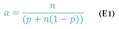
In Equation 1, a is the application speedup, n is the number of processors, and p is the “parallel fraction” of the application (i.e., the fraction of the application that is parallelizable), ranging from 0 to 1. Equations are nice, but understanding how they work and what they tell us is even more important. To do this, examine the extremes in the equation and see what speedup a can be achieved.
In an absolutely perfect world, the parallelizable fraction of the application is p = 1, or perfectly parallelizable. In this case, Amdahl’s Law reduces to a = n. That is, the speedup is linear with the number of cores and is also infinitely scalable. You can keep adding processors and the application will get faster. If you use 16 processors, the application runs 16 times faster. It also means that with one processor, a = 1.
At the opposite end, if the code has a zero parallelizable fraction (p = 0), then Amdahl's Law reduces to a = 1, which means that no matter how many cores or processes are used, the performance does not improve (the wall clock time does not change). Performance stays the same from one processor to as many processors as you care to use.
In summary, if the application cannot be parallelized, the parallelizable fraction is p = 0, the speedup is a = 1, and application performance does not change. If your application is perfectly parallelizable, p = 1, the speedup is a = n, and the performance of the application scales linearly with the number of processors.
Further Exploration
To further understand how Amdahl’s Law works, take a theoretical application that is 80% parallelizable (i.e., 20% cannot be parallelized). For one process, the wall clock time is assumed to be 1,000 seconds, which means that 200 seconds of the wall clock time is the serial portion of the application. From Amdahl’s Law, the minimum wall clock time the application can ever achieve is 200 seconds. Figure 1 shows a plot of the resulting wall clock time on the y-axis versus the number of processes from 1 to 64.
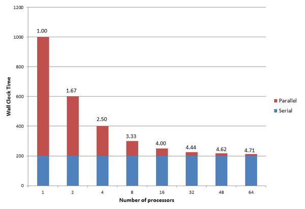 Figure 1: The influence of Amdahl’s Law on an 80% parallelizable application.
The blue portion of each bar is the application serial wall clock time and the red portion is the application parallel wall clock time. Above each bar is the speedup a by number of processes. Notice that with one process, the total wall clock time – the sum of the serial portion and the parallel portion – is 1,000 seconds. Amdahl’s Law says the speedup is 1.00 (i.e., the starting point).
Notice that as the number of processors increases, the wall clock time of the parallel portion decreases. The speedup a increases from 1.00 with one processor to 1.67 with two processors. Although not quite a doubling in performance (a would have to be 2), about one-third of the possible performance was lost because of the serial portion of the application. Four processors only gets a speedup of 2.5 – the speedup is losing ground.
This “decay” in speedup continues as processors are added. With 64 processors, the speedup is only 4.71. The code in this example is 80% parallelizable, which sounds really good, but 64 processors only use about 7.36% of the capability (4.71/64).
As the number of processors increases to infinity, you reach a speedup limit. The asymptotic value of a = 5 is described by Equation 2:
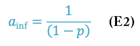
Recall the parallelizable portion of the code is p. That means the serial portion is 1 – p, so the asymptote is the inverse of the serial portion of the code, which controls the scalability of the application. In this example, p = 0.8 and (1 – p) = 0.2, so the asymptotic value is a = 5.
Further examination of Figure 1 illustrates that the application will continue to scale if p > 0. The wall clock time continues to shrink as the number of processes increases. As the number of processes becomes large, the amount of wall clock time reduced is extremely small, but it is non-zero. Recall, however, that applications have been observed to have a scaling limit, after which the wall clock time increases. Why does Amdahl’s Law say that the applications can continue to reduce wall clock time?