
Where does your job data go? The answer is fairly straightforward, but I add some color by throwing in a little high-level background about what resource managers are doing and evolve the question to include a discussion of where data “should” or “could” go.
Where Does Job Output Go?
The second question I need to answer from the top three storage questions a friend sent me is “How do you know where data is located after a job is finished?” The is an excellent question that HPC users who use a resource manager (job scheduler) should contemplate. The question is straightforward to answer, but the question also opens a broader, perhaps philosophical question: Where “should” or “could” your data be located when running a job (application)?
To answer the question with a little background, I’ll start with the idea of a “job.” Assume you run a job with a resource manager such as Slurm. You create a script that runs your job – this script is generically referred to as a “job script” – and submit the job script to the resource manager with a simple command, creating a “job.” The job is then added to the job queue controlled by the resource manager. Your job script can define the resources you need; set up the environment; execute commands, including defining environment variables; execute the application(s); and so on. When the job finishes or the time allowed is exceeded, the job stops and releases the resources.
As resources change in the system (e.g., nodes become available), the resource manager checks the resource requirements of the job, along with any internal rules that have been defined about job priorities, and determines which job to run next. Many times, the rule is simply to run the jobs in the order they were submitted – first in, first out (FIFO).
When you submit your job script to the “queue,” creating the job, the resource manager holds the details of the job script and a few other items, such as details of the submit command that was used. After creating the job, you don’t have to stay logged in to the system; the resource manager runs the job on your behalf.
The resource manager runs the job (job script) on your behalf when the resources you requested are available and it’s your turn to run a job. In general, these are jobs that don’t require any user interaction; they are simply run and the resources are released when it’s done.
However, you can create interactive jobs in which the job script sets up an interactive environment and returns a prompt to a node from the resource manager. When this happens, you can execute whatever commands or scripts or binaries you want. Today, one common interactive application is a Jupyter Notebook. When you exit the node or your allocated time runs out, the job is done and the resources are returned to the resource manager. If you choose to run interactive jobs, be sure to save your data often; otherwise, when the resource manager takes back the resources, you could lose some work.
Because the job, regardless of its type, is executed for you, it is important that you tell the resource manager exactly what resources you need. For example, how many nodes do you need? How many cores per node do you want? Do you need any GPUs or special resources? How much time do you think it will take to complete the job? Equally important is explaining in your job script any special options pertaining to how the job script should be run and the location of the input and output data that the resource manager creates.
If your job script or your application doesn’t specify data locations, then Slurm will accept all input data to be in the directory where you created the job, along with all the output. You will see this referred to as pwd (present working directory), which refers to the directory in which you submitted the job script. (Slurm captures the pwd information.) Of course, the application can specify specific paths to the input data and the paths where it will create the output data. These paths can be hard coded in the application; many times, the application will read environment variables that tell it where to perform the I/O.
In general, if the job script or the application doesn’t specify the location of the input and output, then all the data will appear in the pwd. Almost always, the resource manager captures the stdout and stderr output and puts in into a resource-manager-defined file. For example, in Slurm this would be something like slurm-.out. But the resource managers let you change the name of this output file in the job script or on the command line when you submit the job script.
I don’t want to dive into the writing of job scripts, but because the resource manager creates an output file for you, or lets you define the name of the file, you can include all kinds of detail of the job in this output file, including dates and times, paths, nodes used, the states of nodes (e.g., how much memory is available), and so on. This information can help document the job details so you can scan through the files to look for specific details. For example, when I first started using a resource manager, one of the engineers on the team created a common definition that we included in the job script to capture the details on the problem examined. It made life so much easier when scanning for details about the simulations.
Overall, that’s it. All data will be read and written to your pwd when you submit your job script to the resource manager. The application or job script can specify other directories with needed data, if you like. If you don’t specify where the input data resides or the name of the output, it will show up as slurm-.out in the pwd where you submitted your job script.
Unless told otherwise, users will almost always submit their jobs from their /home directory, meaning all the input and output data will be located there. As users are added, as projects grow, and as the applications require more input data, this arrangement might be untenable because of the capacity limits and performance limits of /home. The cluster admin can impose quotas that help control the growth of data and suggest compressing data files to save space. In the end, capacity is finite.
Additionally, storage has a fixed performance limit, and the more users sharing that resource, the more the effective performance that each user can get goes down, possibly reducing application performance. At some point cluster admins and users start wondering whether they don’t have a better way to organize their data, application data, and so on.
Where To Run Jobs
The obvious answer to needing more storage capacity and possibly performance is simply to buy more. Your storage solution can add capacity and performance easily, right? However, notice that this is a single tier of storage; that is, all the storage has the same performance for all the data.
If you need more performance, you just buy a faster storage solution or add more storage hardware (e.g., more storage servers). Sometimes this can be done without adding much (any?) additional capacity and almost always means that the cost per gigabyte increases, so the overall cost for the same amount of space goes up. I’ve never seen storage solution costs go down with faster performance.
At some point you will have to balance the almost insatiable appetite for more storage capacity and the need for faster storage to run applications effectively. What HPC data centers have done to help address this problem is to examine what is happening with the data.
Usually, the results of the examination are twofold:
- The “age” distribution of the user data skews older; that is, a significant portion of the data is older and hasn’t been touched or used for a long time, compared with other data that is actively used.
- Many applications don’t need extreme storage performance to run effectively. They can run using slower performance storage with little effect on applications.
From these observations, questions start popping up. Does the old data that hasn’t been used in a long time need access to storage with very high performance? Why not put this data on slower storage that has a much greater capacity and has a much lower cost per gigabyte? It seems logical to create different pools of storage that each have very different characteristics.
This approach is called “tiering” storage, in which a small amount of really fast storage with a large cost per gigabyte is purchased. The savings come because you don’t need to buy a huge amount. Instead, you buy a great deal more storage that has much less performance but also has a much smaller cost per gigabyte, allowing for much more capacity. This slower storage has the tongue-in-cheek title of “cheap and deep” (low-cost and lots of it).
Compared with the original single tier of storage where you had to balance capacity and cost so that neither requirement was really satisfied, this new approach of tiered storage – with a much smaller amount of storage that is has much greater performance than before, along with huge amounts of “cheap and deep” storage that is much less expensive and has massive capacity – can produce a much better overall solution satisfying, to some extent, the two extremes: performance and capacity.
Of course, tiering introduces complications. You have to worry about copying data from one of the slower tiers to the fastest tier, run the applications, and copy the data back to the slower tier; that is, you save the capacity of the fastest tier for jobs that are actively running or soon will run applications. To perform this data migration, users must learn about the commands and tools needed for the manual intervention, which, by virtue of being manual, is prone to mistakes.
Combining the storage tiers into one seemingly unified storage space or using “automatic” tools to migrate data has not had much success because the processes that users develop to perform their work are so diverse that no single tool is sufficient. Creating a new type of filesystem with tiers is a very non-trivial task. Therefore, most sites stick with manual data migration by users, but they really focus on training and developing any sort of tool to make the task easier.
Another complication that arises with manual data migration is that the admin needs to police the fast-tier storage, so users don’t forget about any data sitting there that isn’t being actively used.
You can have as many tiers as you like. Many larger HPC systems have perhaps three tiers (Figure 1). The top tier has the fastest performance with the smallest capacity (greatest $/GB). The second tier holds the /home directories for users, with less performance than the top tier but a much larger capacity (smaller $/GB than the top tier). The third tier has very little performance but has massive capacity (smallest $/GB).
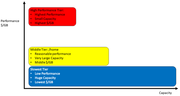 Figure 1: Three tiers of storage are approximately placed in the chart according to their performance. The width of the block is relative to the capacity of that tier. Travel up the y-axis for increased performance and cost per gigabyte. Go right along the x-axis for increased capacity.
Storage Tiering with Local Node Storage
When HPC clusters first became popular, each node used a single disk to hold the operating system (OS) that was just large enough for the OS and anything else needed locally on the node. These drives could be a few gigabytes in capacity, perhaps 4GB, or about double that capacity. Linux distributions, especially those used in HPC, did not require much space. Consequently, the unused capacity in these drives was quite large.
This leftover space could be used for local I/O on the node, or you could use this extra space in each node to create a distributed filesystem (e.g., a parallel virtual filesystem (PVFS) which is now known as OrangeFS) that is part of the kernel. Applications could then use this shared space to, perhaps, access better performing storage to improve performance.
Quite a few distributed applications, primarily the message passing interface (MPI), only had one process – the rank 0 process – perform I/O. Consequently, a shared filesystem wasn’t needed, and I/O could happen locally on one node.
For many applications, local node storage provided enough I/O performance that the overall application runtime was not really affected, allowing applications that were sensitive to I/O performance to use the presumably faster shared storage. Of course, when using the local node storage, the user had to be cognizant of having to move the files onto and off of the local storage to something more permanent.
Over time, drives kept getting larger and the cost per gigabyte dropped rapidly. Naturally, experiments were tried that put several drives in the local node and used a hardware-based RAID controller to combine them as needed. This approach allowed applications with somewhat demanding I/O performance requirements to continue to use local storage and worked well, but for a few drawbacks:
- The cost of the hardware RAID card and extra drives could notably add to the node cost.
- The performance of the expansion slot that held the RAID card could limit storage performance, or the controller’s capability could limit performance.
- Hard drives failed more often than desired, forcing the need for keeping spares on hand and thus adding to the cost.
As a result, many times only a small subset of nodes had RAID-enabled local storage.
As time progressed, I noticed three trends. The first is that CPUs gained more and more cores and more performance, allowing some of the cores to be used for RAID computations (so-called software RAID) so that hardware-based RAID cards were not needed, saving money, and improving performance.
The second trend was systems with much more memory than ever before could be used in a variety of ways (e.g., for caching filesystem data, although at some risk). In the extreme, you could even create a temporary RAM disk – system memory made to look like a storage device – that could be used for storage.
The third trend is that the world now had solid-state drives (SSDs) that were inexpensive enough to put into compute nodes. These drives had much greater performance than hard drives, making them very appealing. Initially the drives were fairly expensive, but over time costs dropped. For example, today you can get consumer-grade 1-2TB SSD drives for well under $100, and I’ve seen some 1TB SSDs for under $30 (August 2023). Don’t forget that SSDs can range from thin 2.5-inch form factors to little NVMe drives that are only a few millimeters thick and very short. The M.2 SSDs are approximately 22mm wide and 60-80mm long. It became obvious that putting a fair number of SSDs that are very fast, very small, and really inexpensive in every node is an easily achievable goal, but what about the economics of this configuration?
With SSD prices dropping and capacities increasing, the cost per gigabyte has dropped rapidly, as well. At the same time, the cost of CPUs and accelerators, such as GPUs, has been increasing rapidly. These computational components of a node now account for the vast majority of the total node cost. Adding a few more SSDs to a node does not appreciably affect the total cost of a node, so why not put in a few more SSDs and use software RAID?
Today you see compute nodes with 4-6 (or more) SSD drives that are combined by software RAID with anything from RAID 0 to RAID 5 or RAID 6. These nodes now have substantial performance in the tens of gigabytes per second range and a capacity pushing 20TB or more. Many (most?) MPI applications still do I/O with the rank 0 process, and this amount of local storage with fantastic performance just begs for users to run their code on local node storage.
Local storage can now be considered an alternative or, at the very least, a partner to the very fast, expensive, top-tier storage solution. Parallel filesystems can be faster than local node storage with SSDs, but the cost, particularly the cost per gigabyte, can be large enough to restrict the total capacity significantly. If applications don’t need superfast storage performance, local storage offers really good performance that is not shared with other users and is less expensive. As before, you have freed the shared really fast storage for applications that need performance better than the local node.
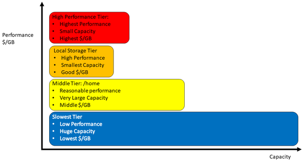 Figure 2: Storage tiering with local storage added.
Figure 2 is the same chart as in Figure 1, but local storage has been added. Note that local storage isn’t quite as fast as the high-performance tier, but it is faster than the middle tier. The local storage tier has a better (lower) cost per gigabyte than the highest performance tier, but it is a bit higher than the middle tier. Overall the local storage tier has less capacity than the other tiers, but that is really the storage per node. Nonetheless, applications can’t access the local storage in other nodes.
Users still have to contend with moving their data to and from the local storage of the compute nodes. (Note that you will always have a user who forgets to copy their data to and copy their data back from the compute node. This is the definition of humanity, but you can’t let this stop the use of this very fast local storage.) Users have had to contend with storage tiers, so adding an option that operationally is the same as before will only result in a little disturbance.
The crux of this section? Buy as much SSD capacity and performance for each compute node as you can, and run your applications on local storage, unless the application requires distributed I/O or massive performance that local nodes cannot provide. The phrase “as you can” generally means to add local storage until the price per node noticeably increases. The point where this occurs depends on your system and application I/O needs.
Summary
The discussion of where the data should or could go started with a little history of shared storage for clusters then sprang into a discussion of storage tiering. Storage tiers are all the rage in the cluster world. They are very effective at reducing costs while still providing great performance for those applications that need it and high capacities for storing data that isn’t used very often but can’t be erased (or the user doesn’t want to erase it).
With the rise of computational accelerators and their corresponding applications, using storage that is local to the compute node has become popular. Putting several SSDs into an accelerated server with software RAID does not appreciably increase the node cost. Moreover, this local storage has some pretty amazing performance that fits into a niche between the highest and middle performance tiers. Many applications can use this storage to their advantage, perhaps reducing the capacity and performance requirements for the highest performance tier.