You just bought a new system with lots and lots of cores (e.g., a desktop with 64 cores or a server with 128 cores). Now that you have all of these cores, why not take advantage of them by parallelizing your code? Depending on your code and your skills, you have a number of paths to parallelization, but after some hard work profiling and lots of testing, your application is successfully parallelized – and it gives you the correct answers! Now comes the real proof: You start checking your application’s performance as you add processors.

Suppose that running on a single core takes about three minutes (180 seconds) of wall clock time. Cautiously, but with lots of optimism, you run it on two cores. The wall clock time is just about two and a half minutes (144 seconds), which is 80% of the time on a single processor. Success!!

You are seeing parallel processing in action, and for some HPC enthusiasts, this is truly thrilling. After doing your “parallelization success celebration dance,” you go for it and run it on four cores. The code runs in just over two minutes (126 seconds). This is 70% of the time on a single core. Maybe not as great as the jump from one to two cores, but it is running faster than a single core. Now try eight cores (more is better, right?). This runs in just under two minutes (117 seconds) or about 65% of the single core time. What?

Now it’s time to go for broke and use 32 cores. This test takes about 110 seconds or about 61% of the single core time. Argh! You feel like Charlie Brown trying to kick the football when Lucy is holding it. Enough is enough: Try all 64 cores. The application takes 205 seconds. This is maddening! Why did the wall clock time go up? What’s going on?

Gene Amdahl

In essence, the wall clock time of an application does not scale with the number of cores (processors). Adding processors does not linearly decrease time. In fact, the wall clock time can increase as you add processors, as it did in the example here. The scalability of the application is limited for some reason: Amdahl’s Law.

In 1967 Gene Amdahl proposed the formula underlying these observed limits of scalability:

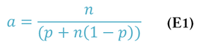
In Equation 1, a is the application speedup, n is the number of processors, and p is the “parallel fraction” of the application (i.e., the fraction of the application that is parallelizable), ranging from 0 to 1. Equations are nice, but understanding how they work and what they tell us is even more important. To do this, examine the extremes in the equation and see what speedup a can be achieved.

In an absolutely perfect world, the parallelizable fraction of the application is p = 1, or perfectly parallelizable. In this case, Amdahl’s Law reduces to a = n. That is, the speedup is linear with the number of cores and is also infinitely scalable. You can keep adding processors and the application will get faster. If you use 16 processors, the application runs 16 times faster. It also means that with one processor, a = 1.

At the opposite end, if the code has a zero parallelizable fraction (p = 0), then Amdahl's Law reduces to a = 1, which means that no matter how many cores or processes are used, the performance does not improve (the wall clock time does not change). Performance stays the same from one processor to as many processors as you care to use.

In summary, if the application cannot be parallelized, the parallelizable fraction is p = 0, the speedup is a = 1, and application performance does not change. If your application is perfectly parallelizable, p = 1, the speedup is a = n, and the performance of the application scales linearly with the number of processors.

Further Exploration

To further understand how Amdahl’s Law works, take a theoretical application that is 80% parallelizable (i.e., 20% cannot be parallelized). For one process, the wall clock time is assumed to be 1,000 seconds, which means that 200 seconds of the wall clock time is the serial portion of the application. From Amdahl’s Law, the minimum wall clock time the application can ever achieve is 200 seconds. Figure 1 shows a plot of the resulting wall clock time on the y-axis versus the number of processes from 1 to 64.

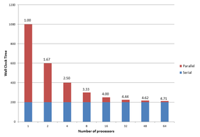
Figure 1: The influence of Amdahl’s Law on an 80% parallelizable application.

The blue portion of each bar is the application serial wall clock time and the red portion is the application parallel wall clock time. Above each bar is the speedup a by number of processes. Notice that with one process, the total wall clock time – the sum of the serial portion and the parallel portion – is 1,000 seconds. Amdahl’s Law says the speedup is 1.00 (i.e., the starting point).

Notice that as the number of processors increases, the wall clock time of the parallel portion decreases. The speedup a increases from 1.00 with one processor to 1.67 with two processors. Although not quite a doubling in performance (a would have to be 2), about one-third of the possible performance was lost because of the serial portion of the application. Four processors only gets a speedup of 2.5 – the speedup is losing ground.

This “decay” in speedup continues as processors are added. With 64 processors, the speedup is only 4.71. The code in this example is 80% parallelizable, which sounds really good, but 64 processors only use about 7.36% of the capability (4.71/64).

As the number of processors increases to infinity, you reach a speedup limit. The asymptotic value of a = 5 is described by Equation 2:

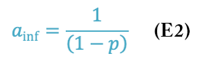
Recall the parallelizable portion of the code is p. That means the serial portion is 1 – p, so the asymptote is the inverse of the serial portion of the code, which controls the scalability of the application. In this example, p = 0.8 and (1 – p) = 0.2, so the asymptotic value is a = 5.

Further examination of Figure 1 illustrates that the application will continue to scale if p > 0. The wall clock time continues to shrink as the number of processes increases. As the number of processes becomes large, the amount of wall clock time reduced is extremely small, but it is non-zero. Recall, however, that applications have been observed to have a scaling limit, after which the wall clock time increases. Why does Amdahl’s Law say that the applications can continue to reduce wall clock time?

Limitations of Amdahl’s Law

The disparity between what Amdahl’s Law predicts and the time in which applications can actually run as processors are added lies in the differences between theory and the limitations of hardware. One such source of the difference is that real parallel applications exchange data as part of the overall computations: It takes time to send data to a processor and for a processor to receive data from other processors. Moreover, this time depends on the number of processors. Adding processors increases the overall communication time.
.

Amdahl’s Law does not account for this communication time. Instead, it assumes an infinitely fast network; that is, data can be transferred infinitely fast from one process to another (zero latency and infinite bandwidth).

Non-zero Communication Time

A somewhat contrived model can illustrate what happens when communication time is non-zero. This model assumes that serial time is not a function of the number of processes, just as does Amdahl’s Law. Additionally, a portion of time is not parallelizable but is also a function of the number of processors, representing the time for communication between processors that increases as the number of processes increases.

To create a model, start with a constraint from Amdahl’s Law that says the sum of the parallelizable fraction p and the non-parallelizable fraction (1 – p) has to be 1:

Remember that in Amdahl’s Law the serial or non-parallelizable fraction is not a function of the number of processors. Assume the serial fraction is:

The constraint can then be rewritten as:

The serial fraction can be broken into two parts (Equation 6), where s_B is the base serial fraction that is not a function of the number of processors, and s_C is the communication time between processors, which is a function of n, the number of processors:

When this equation is substituted back into Amdahl’s Law, the result is Equation 8 for speedup a:

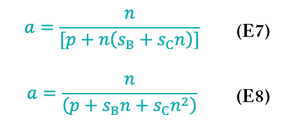
Notice that the denominator is now a function of n².

From Equation 8 you can plot the speedup. As with the previous problem, assume a parallel portion p = 0.8, leaving a serial portion s = 0.2. Assigning the base serial portion s_B = 0.195, independent of n, leaves the communication portion s_C = 0.005. Figure 2 shows the plot of speedup a as a function of the number of processors.

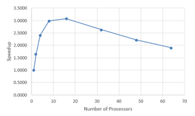
Figure 2: Speedup with new model.

Notice that the speedup increases for a bit but then decreases as the number of processes increases, which is the same thing as increasing the number of processors and increasing the wall clock time.

Notice that the peak speedup is only about a = 3.0 and happens at around 16 processors. This speedup is less than that predicted by Amdahl’s Law (a = 5). Note that you can analytically find the number of processors for the peak speedup by taking the derivative of the equation plotted in Figure 2 with respect to n and setting it to 0. You can then find the speedup from the peak value of n. I leave this exercise to the reader.

Although the model is not perfect, it does illustrate how the application speedup can decrease as the number of processes increase. On the basis of this model, you can say, from a higher perspective, that the equation for a must have a term missing that perhaps Amdahl’s Law doesn’t show that is a function of the number of processes causing the speedup to decrease with n.

Some other attempts have been made to account for non-zero communication time in Amdahl’s Law. One of the best is from Bob Brown at Duke. He provides a good analogy of Amdahl’s Law that includes communication time in some fashion.

Another assumption in Amdahl’s law drove the creation of Gustafson’s Law. Whereas Amdahl’s Law assumes the problem size is fixed relative to the number of processors, Gustafson argues that parallel code is run by maximizing the amount of computation on each processor, so Gustafson’s Law assumes that the problem size increases as the number of processors increases. Thus, solving a larger problem in the same amount of time is possible. In essence, the law redefines efficiency.

You can use Amdahl’s Law, Gustafson’s Law, and derivatives that account for communication time as a guide to where you should concentrate your resources to improve performance. From the discussion about these equations, you can see that focusing on the serial portion of an application is an important way to improve scalability.

Origin of Serial Compute Time

Recall that the serial portion of an application is the compute time that doesn’t change with the number of processors. The parts of an application that contribute to the serial portion of the overall application really depend on your application and algorithm. Serial performance has several sources, but usually a predominant source is I/O. When an application starts, it most likely needs to read an input file so that all of the processes have the problem information. Some applications also need to write data at some point while it runs. At the end, the application will likely write the results.

Typically these I/O steps are accomplished by a single process to avoid collisions when multiple processes do I/O, particularly writes. If two processes open the same file, try to write to it, and the filesystem isn’t designed to handle multiple writes, the data might be written incorrectly. For example, if process 1 is supposed to write data first, followed by process 2, what happens if process 2 writes first followed by process 1? You get a mess. However, with careful programming, you can have multiple processes write to the same file. As the programmer, you have to be very careful that each process does not try to write where another process is writing, which can involve a great deal of work.

Another reason to use a single process for I/O is ease of programming. As an example, assume an application is using the Message Passing Interface (MPI) library to parallelize code. The first process in an MPI application is the rank 0 process, which handles any I/O on its own. For reads, it reads the input data and sends it to other processes with MPI_Send, MPI_Isend, or MPI_Bcast from the rank 0 process and with MPI_Recv, MPI_Irecv, or MPI_Bcast, for the non-rank-0 processes. Writes are the opposite: The non-rank-0 processes send their data to the rank 0 process, which does the I/O on behalf of all processes.

Having a single MPI process do the I/O on behalf of the other processes by exchanging data creates a serial bottleneck in your application because only one process is doing I/O, forcing the other processes to wait.

If you want your application to scale, you need to reduce the amount of serial work done by the application, including moving data to or from processes. You have a couple of ways to do this. The first, which I already mentioned, is to have each process do its own I/O. This approach requires careful coding, or you can accidentally corrupt data file(s).

The most common way is to have all the processes perform I/O with MPI-IO. This is an extension of MPI that was incorporated in MPI-2 and allows I/O from all MPI processes in an application (or a subset of the processes). It is beyond the scope of this article to discuss MPI-IO, but remember it can be a tool to help you reduce the serial portion of your application by parallelizing the I/O.

Before you undertake a journey to modify your application to parallelize the I/O, you should understand whether I/O is a significant portion of the total application runtime. If the I/O portion is fairly small –where the definition of “fairly small” is up to you – it might not be worth your time to rewrite the I/O portion of the application. In a previous article I discuss various ways to profile the I/O of your application.

If serial I/O is not a significant portion of your application, you might need to look for other sources of serialized performance. Tracking down these sources can be difficult and tedious, but it is usually worthwhile because it improves the scalability and performance of the application – and who doesn’t like speed?

Summary

Writing a useful parallel application is a great accomplishment. At some point you will want to try running the application with larger core counts to improve performance, which is one of the reasons you wrote a parallel application in the first place. However, when at some point increasing the number of processors used in the application stops decreasing and starts increasing the wall clock time of the application, it’s time to start searching for reasons why this is happening.

The first explanation is from Amdahl’s Law, which illustrates the theoretical speedup of an application when running with more processes and the limitation of serial code on wall clock time. Although it can be annoying that parallel processing is limited by serial performance and not something directly involving parallel processing, it does explain that at some point, your application will not run appreciable faster unless your application has a very small serial portion.

The second explanation for decreased performance is serial bottlenecks in an application caused by I/O. Examining the amount of time an application spends on I/O is an important step in understanding the serial portion of your application. Luckily you can find tools and libraries to parallelize the application I/O; however, at some fundamental level, the application has to do some I/O to read input and write output, limiting the scalability of the application (scalability limit).

The goal is to push this scalability limit to the largest number of processes possible, so get out there and improve the serial portion of your applications!