
I/O Characterization of TensorFlow with Darshan
Darshan I/O Analysis for Deep Learning Frameworks
The Darshan userspace tool is often used for I/O profiling of HPC applications. It is broken into two parts: The first part, darshan-runtime, gathers, compresses, and stores the data. The second part, darshan-util, postprocesses the data.
Darshan gathers its data either by compile-time wrappers or dynamic library preloading. For message passing interface (MPI) applications, you can use the provided wrappers (Perl scripts) to create an instrumented binary. Darshan uses the MPI profiling interface of MPI applications for gathering information about I/O patterns. It does this by “… injecting additional libraries and options into the linker command line to intercept relevant I/O calls.”
For MPI applications, you can also profile pre-compiled binaries. It uses the LD_PRELOAD environment variable to point to the Darshan shared library. This approach allows you to run uninstrumented binaries for which you don’t have the source code (perhaps independent software vendor applications) or applications for which you don’t want to rebuild the binary.
For non-MPI applications you have to use the LD_PRELOAD environment variable and the Darshan shared library.
Deep Learning (DL) frameworks such as TensorFlow are becoming an increasingly big part of HPC workloads. Because one of the tenets of DL is using as much data as possible, understanding the I/O patterns of these applications is important. Terabyte datasets are quite common. In this article, I want to take Darshan, a tool based on HPC and MPI, and use it to examine the I/O pattern of TensorFlow on a small problem – one that I can run on my home workstation.
Installation
To build Darshan for non-MPI applications, you should set a few options when building the Darshan runtime (darshan-runtime). I used the configure command:
./configure --with-log-path=/home/laytonjb/darshan-logs \
            --with-jobid-env=NONE \
            --enable-mmap-logs \
            --enable-group-readable-logs \
            --without-mpi CC=gcc \
            --prefix=[binary location]
Because I’m the only one using the system, I put the Darshan logs (the output from Darshan) in a directory in my home directory (/home/laytonjb/darshan-log), and I installed the binaries into my /home directory (not good ideas for multiuser systems). This script preps the environment and creates a directory hierarchy in the log directory (the one specified when configuring Darshan). The organization of the hierarchy is simple. The top-most directory is the year. Below that is the month. Below that is the day.
After the usual, make; make install, you should run the command:
darshan-mk-log.pl
This command preps the log directory. For multiuser systems, you should read the documentation. Next, I built the Darshan utilities (darshan-util) with the command:
./configure CC=gcc --prefix=[binary location]
I’m running these tests on an Ubuntu 20.04 system. I had to install some packages for the postprocessing (darshan-util) tools to work:
texlive-latex-extralibpod-latex-perl
Different distributions may require different packages. If you have trouble, the Darshan mailing list is awesome. (You’ll see my posts where I got some help when I was doing postprocessing).
Simple Example
Before jumping into Darshan with a DL example, I want to test a simple example so I can get a feel for the postprocessing output. I grabbed an example from a previous article (Listing 1). Although this example doesn’t produce much I/O, I was curious to see whether Darshan could profile the I/O the application does create.
Listing 1: I/O Example Code
program ex1

    type rec
        integer :: x, y, z
        real :: value
    end type rec

    integer :: counter
    integer :: counter_limit
    integer :: ierr

    type(rec) :: my_record

    counter_limit = 2000

    ierr = -1
    open(unit=8,file="test.bin", status="replace", &
         action="readwrite", &
         iostat = ierr)
    if (ierr > o) then
        write(*,*) "error in opening file Stopping"
        stop
    else
        do counter = 1,counter_limit
            my_record%x = counter
            my_record%y = counter + 1
            my_record%z = counter + 2
            my_record%value = counter * 10.0
            write(8,*) my_record
        end do
    end if

    close(8)

end program ex1
For this example, the command I used for Darshan to gather I/O statistics on the application was:
env LD_PRELOAD=/home/laytonjb/bin/darshan-3.3.1/lib/libdarshan.so ./ex1
I copied the Darshan file from the log location to a local directory and ran the Darshan utility darshan-job-summary.pl against the output file. The result is a PDF file that summarizes the I/O of the application.
Rather than include the entire PDF file in this article, I grabbed some of the plots and tables and present them here. Figure 1 shows a quick summary at the beginning of the output and says that it measured 0.1MiB of I/O. It also estimates the I/O rate at 544.77MiBps.
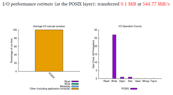 Figure 1: I/O performance from darshan-job-summary.pl output PDF.
The left-hand chart presents the percentage of runtime for read, write, and metadata I/O and computation. For this case, it shows that the runtime is entirely dominated by computation. The read, write, and metadata bars are negligible and really can’t even be seen.
The chart on the right presents the number of specific I/O operations, with one open operation and 27 write operations. It also shows that all of the I/O is done by POSIX I/O functions.
The next snippet of the summary PDF is shown in the histogram in Figure 2, a plot of the typical payloads for read and write function calls (i.e., how many function calls use how much data per read or write per I/O function call). This chart shows that all of the write payloads are between 1 and 10KiB and that this example had no reads.
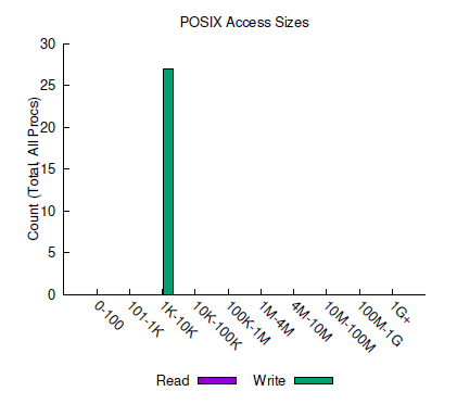 Figure 2: Access sizes in darshan-job-summary.pl output PDF.
The job summary from Darshan also creates some very useful tables (Figure 3). The table on the left presents the most common payload sizes for POSIX I/O functions, with two access sizes, 4104 and 1296 bytes. The table on the right presents file-based I/O stats. Only one file was involved in this really simple example, and it was a write-only file. Note that the Darshan summary matches the source code; the one and only file was opened as write only. The table also shows that the average size of the file was 106KiB (the same as the maximum size).
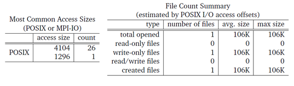 Figure 3: Job summary tables from darshan-job-summary.pl output PDF.
Another group of useful tables are shown in Figure 4. The top table presents the cumulative time spent in reads and writes for both independent and shared operations. Don’t forget that Darshan’s origins are in MPI and HPC I/O, where shared files are common. It also presents information on how much I/O was performed for both reads and writes. Notice that the write time was really small (0.000127 seconds), and the I/O was also very small (0.103MiB).
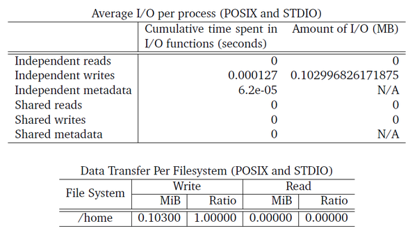 Figure 4: I/O stats from darshan-job-summary.pl output PDF.
Darshan also shows a great stat in the amount of time spent on metadata. Just focusing on the read and write performance is not quite enough for understanding I/O performance. Metadata I/O can have a big effect on I/O, and separating it out from reads and writes is very useful.
The bottom table gives the total I/O for the various filesystems. This table is a bit more useful for HPC applications that may use a scratch filesystem for I/O and a filesystem for storing the application binaries. Increasingly, DL applications are using this approach, so examining this table is useful.
The last snippet of the job summary I want to highlight is the number of read/write I/O operations (Figure 5). The figure shows only write operations, as expected. The total operations include all I/O functions.
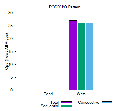 Figure 5: Read/write operations from the darshan-job-summary.pl output PDF.
Darshan with TensorFlow
Darshan has had a number of successes with MPI applications. For this article, I wanted to try it on a TensorFlow framework, with Keras loading the data, creating the model, training the model for only 100 epochs, checkpointing after every epoch, and saving the final model.
The system I’ll be using is my home workstation with a single Titan V card, a six-core AMD Ryzen CPU, and 32GB of memory. I plan to use the CIFAR-10 data and use the training code from Jason Brownlee’s Machine Learning Mastery website (How to Develop a CNN From Scratch for CIFAR-10 Photo Classification. Accessed July 15, 2021). I’ll start the training from the beginning (no pre-trained models) and run it for 100 epochs. I've updated the training script to checkpoint the model weights after every epoch to the same file (it just overwrites).
The code is written in Python and uses Keras as the interface to TensorFlow. Keras is great for defining models and training. I used the individual edition of Anaconda Python for this training. The specific software versions I used were:
- Ubuntu 20.04
- Conda 4.10.3
- Python 3.8.10
- TensorFlow 2.4.1
- cudatoolkit 10.1.243
- System CUDA 11.3
- Nvidia driver 465.19.01
A summary of the model is shown in Table 1, with a total of six convolution layers, a maximum of three pooling layers, and the final flattening layer followed by a fully connected layer (dense) that connects to the final output layer for the 10 classes.
Table 1: Training Model
| Layer (type) | Output Shape | No. of Parameters |
| conv2d (Conv2D) | (None, 32, 32, 32) | 896 |
| conv2d_1 (Conv2D) | (None, 32, 32, 32) | 9,248 |
| max_pooling2d (MaxPooling2D) | (None, 16, 16, 32) | 0 |
| conv2d_2 (Conv2D) | (None, 16, 16, 64) | 18,496 |
| conv2d_3 (Conv2D) | (None, 16, 16, 64) | 36,928 |
| max_pooling2d_1 (MaxPooling2) | (None, 8, 8, 64) | 0 |
| conv2d_4 (Conv2D) | (None, 8, 8, 128) | 73,856 |
| conv2d_5 (Conv2D) | (None, 8, 8, 128) | 147,584 |
| max_pooling2d_2 (MaxPooling2) | (None, 4, 4, 128) | 0 |
| flatten (Flatten) | (None, 2048) | 0 |
| dense (Dense) | (None, 128) | 262,272 |
| dense_1 (Dense) | (None, 10) | 1,290 |
| Total parameters | 550,570 | |
| Trainable parameters | 550,570 | |
| Non-trainable parameters | 0 |
The first two convolutional layers have 32 filters each, the second two convolutional layers have 64 filters each, and the final two convolutional layers have 128 filters each. The maximum pooling layers are defined after every two convolution layers with a 2x2 filter. The fully connected layer has 128 neurons. The total number of parameters is 550,570 (a very small model).
The command to run the training script with Darshan is shown in Listing 2. Running the training script takes several lines, so I just put them into a Bash script and run that.
Listing 2: Training Script
export DARSHAN_EXCLUDE_DIRS=/proc,/etc,/dev,/sys,/snap,/run,/user,/lib,/bin,/home/laytonjb/anaconda3/lib/python3.8,/home/laytonjb/bin,/tmp
export DARSHAN_MODMEM=20000
env LD_PRELOAD=/home/laytonjb/bin/darshan-3.3.1/lib/libdarshan.so python3 cifar10-4.checkpoint.py
When the training script is run, Python starts and Python modules are loaded, which causes a large number of Python modules to be converted (compiled) to byte code (.pyc files). Darshan can currently only monitor 1,024 files during the application run, and running the training script exceeded this limit. Because most of the files being compiled were Python modules, the Python directory (/home/laytonjb/anaconda3/lib/python3.8) had to be excluded from the Darshan analysis. Other directories were excluded, too, because they don’t contribute much to the overall I/O and could cause Darshan to exceed the 1,024-file limit. The first line of the script excludes specific directories.
The second line in the script increases the amount of memory the Darshan instrumentation modules can collectively use at runtime. By default, the amount of memory is 2MiB, but I allowed 19.53GiB (20GB) to make sure I gathered the I/O data.
Remember that the Darshan runtime just collects the I/O information during the run. It does not calculate any statistics or create a summary. After it collects the information and the application is finished, the Darshan utilities can be run. I used the darshan-job-summary.pl tool to create a PDF summary of the analysis.
The very top of the PDF file (Figure 6) gives you some quick highlights of the analysis. The top line in the output says that one processor was used, and it took 1,404 seconds for the application to complete. You can also see that the POSIX interface (the POSIX I/O functions) transferred 770.9MiB of data at 416.94MiBps. The STDIO interface (STDIO I/O functions) transferred 0.0MiB at 33.46MiBps. The amount of data transferred through the STDIO interface was so small that the output shows 0.0MiB, which would indicate less than 0.499MiB of data (the code would round this down to one decimal place, or 0.0).
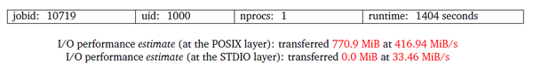 Figure 6: Analysis highlights from the darshan-job-summary.pl output PDF.
The first snippet of the job summary is shown in Figure 7. The top left-hand chart shows that virtually all of the POSIX and STDIO runtime is for computation. You can see a little bit of I/O at the very bottom of the POSIX bar (the left bar in the chart).
The top right-hand chart shows very little STDIO (green bars). The rest is POSIX I/O, dominated by writes. Recall that Darshan has to be run excluding any I/O in the directory /home/laytonjb/anaconda3/lib/python3.8 (the location of Python).
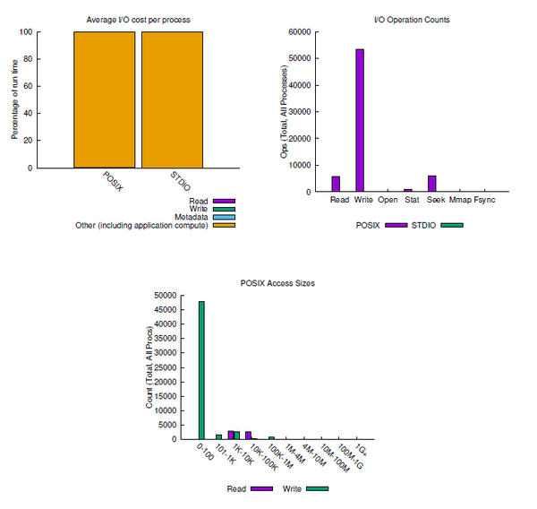 Figure 7: Read/write operations from darshan-job-summary.pl output PDF.
When the training script is executed, Python will go through and convert (compile) Python source code to byte code (.pyc extension) by reading the code (reads) and writing the byte code (writes). This I/O is not captured by Darshan. One can argue whether this is appropriate or not because this conversion is part of the total training runtime. On the other hand, excluding that I/O focuses the Darshan I/O analysis on the training and not Python.
About 54,000 write operations occur during the training (recall that a checkpoint is written after every epoch). About 6,000 read operations appeared to have occurred during the training, which seems to be counterintuitive because DL training involves repeatedly going through the dataset in a different order for each epoch. Two things affect this: (1) TensorFlow has an efficient data interface that minimizes read operations; (2) all of the data fits into GPU memory. Therefore, you don’t see as many read operations as you would expect.
A few metadata operations take place during the training. The top-right chart records a very small number of open and stat operations, as well as a number of lseek operations – perhaps 7,500. Although there doesn’t appear to be a noticeable number of mmap or fsync operations, if Darshan puts them in the chart, that means there are a non-zero number of each.
The bottom chart in Figure 7 provides a breakdown of read and write operations for the POSIX I/O functions. The vast majority of write operations are in the range of 0–100 bytes. A much smaller number of write operations occur in other ranges (e.g., some in the 101 bytes to 1KiB and in the 1–10KiB ranges, and a very small number in the 10–100KiB and the 100KiB to 1MiB ranges). All of the ranges greater than 100 bytes have a much small number of write operations than the lowest range.
A small number of read operations are captured in that specific chart. Most read operations appear to be in the 1–10KiB range, with a few in the 10–100KiB range.
Notice that for both reads and writes, the data per read or write operation is small. A rule of thumb for good I/O performance is to use the largest possible read or write operations, preferably in the mebibyte and greater range. The largest part of the operations for this DL training is in the 1–100 byte range, which is very small.
Figure 8 presents two tables. The left-hand table shows the most common access sizes for POSIX operations. For reads and writes, this is the average size of the data per I/O function call. The right-hand chart presents data on the files used during the run.
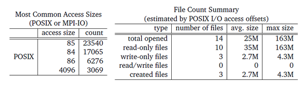 Figure 8: Access sizes and file counts from darshan-job-summary.pl output PDF.
The left-hand table shows that the vast majority of POSIX operations, predominately writes with a small number of reads, are in the 84–86 byte range. These account for 46,881 operations of the roughly 50,000 read and write operations (about 94%). This table reinforces the observation from the charts in Figure 7.
The right-hand table shows that 14 files were opened, of which 10 were read-only and three were write-only. The average size of the files was 25MiB.
The next two tables (Figure 9) present more information about the amount of I/O. The top table first shows the amount of time spent doing reads, writes, and metadata. For the DL training problem, 0.063 seconds was spent on reads, 0.44 seconds on writes, and 1.35 seconds on metadata (non-read and -write I/O operations), or a total of 1.8491 seconds spent on some type of I/O out of 1,404 seconds of runtime (0.13%), which illustrates that this problem is virtually 100% dominated by computation.
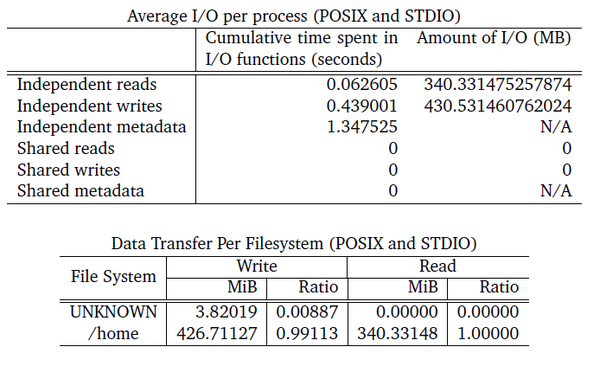 Figure 9: STDIO and POSIX I/O from darshan-job-summary.pl output PDF.
The last column of the top table also presents the total amount of I/O. The read I/O operations, although only a very small number, total 340MiB. The write operations, which dominated the reads, total only 430MiB. These results are very interesting, considering the roughly nine write I/O operations for every read operation.
Finally, the DL training has no shared I/O, so you don’t see any shared reads, writes, or metadata in the top table. Remember that Darshan’s origins are in the HPC and MPI world, where shared I/O operations are common, so it will present this information in the summary.
The bottom table presents how much I/O was done for the various filesystems. A very small amount of I/O is attributed to UNKNOWN (0.887%), but /home (except for /home/laytonjb/anaconda3, which was excluded from the analysis) had 99.1% of the write I/O and 100% of the read I/O.
The final snippet of Darshan output is in Figure 10, where the I/O operation sequences are presented. The chart shows roughly 54,000 total write and perhaps 6,000 total read operations. For the write I/O, most were sequential (about 52,000), with about 47,000 consecutive operations.
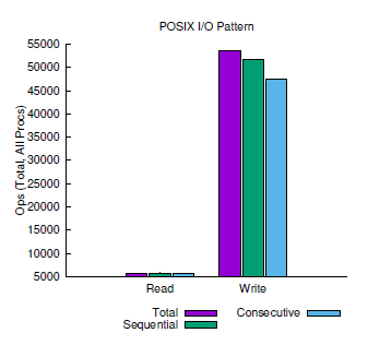 Figure 10: I/O operation sequences from darshan-job-summary.pl output PDF.
Summary
A small amount of work has taken place in the past characterizing or understanding the I/O patterns of DL frameworks. In this article, Darshan, a widely accepted I/O characterization tool rooted in the HPC and MPI world, was used to examine the I/O pattern of TensorFlow running a simple model on the CIFAR-10 dataset.
Deep Learning frameworks that use the Python language for training the model open a large number of files as part of the Python and TensorFlow startup. Currently, Darshan can only accommodate 1,024 files. As a result, the Python directory had to be excluded from the analysis, which could be a good thing, allowing Darshan to focus more on the training. However, it also means that Darshan can’t capture all of the I/O used in running the training script.
With the simple CIFAR-10 training script, not much I/O took place overall. The dataset isn’t large, so it can fit in GPU memory. The overall runtime was dominated by compute time. The small amount of I/O that was performed was almost all write operations, probably writing the checkpoints after every epoch.
I tried larger problems, but reading the data, even if it fit into GPU memory, led to exceeding the current 1,024-file limit. However, the current version of Darshan has shown that it can be used for I/O characterization of DL frameworks, albeit for small problems.
The developers of Darshan are working on updates to break the 1,024-file limit. Although a Python postprocessing capability exists today, the developers are also rapidly updating that capability. Both developments will greatly help the DL community in using Darshan.