Lead Image © Lucy Baldwin, 123RF.com

Lead Image © Lucy Baldwin, 123RF.com

Planning Performance Without Running Binaries

Blade Runner

Article from ADMIN 61/2021
By
We examine some mathemagical tools that approximate time-to-execute given the parallelizable segment of code.

Usually the task of a performance engineer involves running a workload, finding its first bottleneck with a profiling tool, eliminating it (or at least minimizing it), and then repeating this cycle – up until a desired performance level is attained. However, sometimes the question is posed from the reverse angle: Given existing code that requires a certain amount of time to execute (e.g., 10 minutes), what would it take to run it 10 times faster? Can it be done? Answering these questions is easier than you would think.

Parallel Processing

The typical parallel computing workload breaks down a problem in discrete chunks to be run simultaneously on different CPU cores. A classic example is approximating the value of pi. Many algorithms that numerically approximate pi are known, variously attributed to Euler, Ramanujan, Newton, and others. Their meaning, not their mathematical derivation, is of concern here. A simple approximation is given by Equation 1.

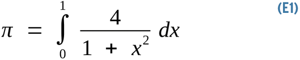
The assertion is that pi is equal to the area under the curve in Figure 1. Numerical integration solves this equation computationally, rather than analytically, by slicing this space into an infinite number of infinitesimal rectangles and summing their areas. This scenario is an ideal parallel numerical challenge, as computing one rectangle's area has no data dependency whatsoever with that of any another. The more the slices, the higher the precision. You just need to throw CPUs at the problem: in this case, 5 million loops to reach 48 decimal places of accuracy.

Figure 1: Approximating pi by numerical integration of the area under the curve.

This way of approximating pi is not very efficient, but it uses a very simple algorithm to implement in both linear and parallel coding styles. Carlos Morrison published a message passing interface (MPI) [1] pi implementation [2] in his book Build Supercomputers with Raspberry Pi 3 [3].

Speed Limit

Can you make the code twice as fast? Sure! Can you make it 10 times faster? Maybe. That factor, 2x or 10x, is called speedup in computing (Equation 2).

Speedup is defined as the ratio of the original and new (hopefully improved) measurements, so if your code used to take one second to execute and now takes half a second, you have a 2x speedup. Speedup measures for latency or throughput – today I am using the latency formulation.

Amdahl's law [4] observes that parallelism only accelerates a fraction of the application's code, putting a limit on its effect. Ideally, speedup would be linear, with a doubling of processing resources consistently halving the compute time, and so on indefinitely. Unfortunately, few algorithms can deliver on this promise (see the "Embarrassingly Parallel Algorithms" box); most algorithms approximate linear speedup over a few CPUs and essentially decay into constant time with many CPUs.

Embarrassingly Parallel Algorithms

An algorithm is considered "embarrassingly parallel" [5] when no design effort is required to partition the problem into completely separate parts. If no data dependency exists between the problem subparts, no communication coordination (and corresponding computational stall) ever takes place, making the problem trivial to partition. Of course, there is nothing embarrassing about using these algorithms – quite the contrary, it is the hallmark of good architecture. Some examples of algorithms in this class, among others, are:

  • Numerical integration – by slice
  • Monte Carlo methods – by sample
  • The Mandelbrot set – by function point
  • Ray tracing or other computer graphics rendering – by frame or ray
  • Genetic algorithms – by genotype
  • Convolutional neural networks – by filter
  • Computer simulation – by scenario

Choosing an efficient parallel algorithm is essential to achieving good return on your hardware or computer time investment.

For example, if your code takes 20 minutes to execute and just one minute of it can't be parallelized, you can tell up front, without knowing any other details about the problem, that the maximum speedup theoretically possible is 20x (Equation 3),

which is derived by observing that you can use as many CPUs as you want to drive 95 percent of the problem asymptotically to zero time (p =0.95), and you will be left with that one minute (1 – p =0.05). Once you do the math (1/0.05=20), that is the maximum possible speedup under ideal conditions (i.e., the absolute limit with infinite resources thrown at the problem).

Amdahl's Law

IBM's Gene Amdahl contributed the law bearing his name in 1967, coupling the previous observation with the simple fact that you generally do not have infinite horsepower to drive the parallel section of the code to zero time (Equation 4).

Amdahl's observation factors in the speedup of the parallel section. The new term p /s is the ratio of time spent in the parallel section of the code and the speedup it achieves.

Continuing with the 20-minute example, say you have accelerated the now-parallel section of the code with a 4x speedup, and you find that the resulting speedup for the whole program is 3.47x (Equation 5):

There are some important observations to be made here. First, accelerating code is usually about removing bottlenecks, not absolute speedup numbers for the whole codebase. Second, given more resources, you will usually process more data or do more work. Gustafson's law [6] provides an alternative formulation: If more resources are made available, larger problems can be solved within the same time, as opposed to Amdahl's law, which analyzes how a fixed workload can be accelerated by adding more resources. Keep these points in mind and remember that, in the real world, network communication is always a distributed system's presumptive bottleneck.

Buy this article as PDF

Express-Checkout as PDF
Price $2.95
(incl. VAT)

Buy ADMIN Magazine

SINGLE ISSUES
 
SUBSCRIPTIONS
 
TABLET & SMARTPHONE APPS
Get it on Google Play

US / Canada

Get it on Google Play

UK / Australia

Related content

  • Why Good Applications Don’t Scale

    You  ha ve parallelized your serial application ,  but as you use more cores you are  n o t seeing any improvement  in performance . What gives?

  • Why Good Applications Don't Scale
    You have parallelized your serial application, but as you use more cores you are not seeing any improvement in performance. What gives?
  • Failure to Scale

    Your parallel application is running fine, but you want it to run faster. Naturally, you use more and more cores, and everything is great; however, suddenly performance starts decreasing. What just happened?

  • Improved Performance with Parallel I/O

    Understanding the I/O pattern of your application is the starting point for improving its I/O performance, especially if I/O is a fairly large part of your application’s run time.

  • Improved Performance with Parallel I/O
    Understanding the I/O pattern of your application is the starting point for improving its I/O performance, especially if I/O is a fairly large part of your application's run time.
comments powered by Disqus
Subscribe to our ADMIN Newsletters
Subscribe to our Linux Newsletters
Find Linux and Open Source Jobs


Support Our Work

ADMIN content is made possible with support from readers like you. Please consider contributing when you've found an article to be beneficial.

Learn More”>
	</a>

<hr>		    
			</div>
		    		</div>

		<div class=