« Previous 1 2 3 Next »
Why Good Applications Don’t Scale
Limitations of Amdahl’s Law
The disparity between what Amdahl’s Law predicts and the time in which applications can actually run as processors are added lies in the differences between theory and the limitations of hardware. One such source of the difference is that real parallel applications exchange data as part of the overall computations: It takes time to send data to a processor and for a processor to receive data from other processors. Moreover, this time depends on the number of processors. Adding processors increases the overall communication time.
.
Amdahl’s Law does not account for this communication time. Instead, it assumes an infinitely fast network; that is, data can be transferred infinitely fast from one process to another (zero latency and infinite bandwidth).
Non-zero Communication Time
A somewhat contrived model can illustrate what happens when communication time is non-zero. This model assumes that serial time is not a function of the number of processes, just as does Amdahl’s Law. Additionally, a portion of time is not parallelizable but is also a function of the number of processors, representing the time for communication between processors that increases as the number of processes increases.
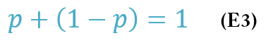
To create a model, start with a constraint from Amdahl’s Law that says the sum of the parallelizable fraction p and the non-parallelizable fraction (1 – p) has to be 1:
Remember that in Amdahl’s Law the serial or non-parallelizable fraction is not a function of the number of processors. Assume the serial fraction is:
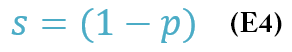
The constraint can then be rewritten as:

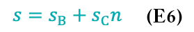
The serial fraction can be broken into two parts (Equation 6), where sB is the base serial fraction that is not a function of the number of processors, and sC is the communication time between processors, which is a function of n, the number of processors:
When this equation is substituted back into Amdahl’s Law, the result is Equation 8 for speedup a:
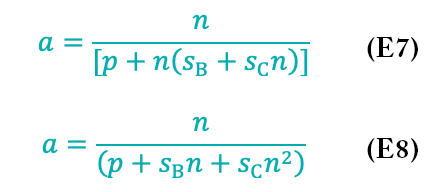
Notice that the denominator is now a function of n2.
From Equation 8 you can plot the speedup. As with the previous problem, assume a parallel portion p = 0.8, leaving a serial portion s = 0.2. Assigning the base serial portion sB = 0.195, independent of n, leaves the communication portion sC = 0.005. Figure 2 shows the plot of speedup a as a function of the number of processors.
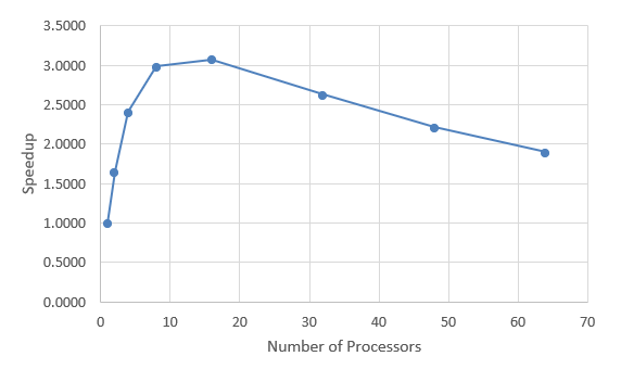 Figure 2: Speedup with new model.
Notice that the speedup increases for a bit but then decreases as the number of processes increases, which is the same thing as increasing the number of processors and increasing the wall clock time.
Notice that the peak speedup is only about a = 3.0 and happens at around 16 processors. This speedup is less than that predicted by Amdahl’s Law (a = 5). Note that you can analytically find the number of processors for the peak speedup by taking the derivative of the equation plotted in Figure 2 with respect to n and setting it to 0. You can then find the speedup from the peak value of n. I leave this exercise to the reader.
Although the model is not perfect, it does illustrate how the application speedup can decrease as the number of processes increase. On the basis of this model, you can say, from a higher perspective, that the equation for a must have a term missing that perhaps Amdahl’s Law doesn’t show that is a function of the number of processes causing the speedup to decrease with n.
Some other attempts have been made to account for non-zero communication time in Amdahl’s Law. One of the best is from Bob Brown at Duke. He provides a good analogy of Amdahl’s Law that includes communication time in some fashion.
Another assumption in Amdahl’s law drove the creation of Gustafson’s Law. Whereas Amdahl’s Law assumes the problem size is fixed relative to the number of processors, Gustafson argues that parallel code is run by maximizing the amount of computation on each processor, so Gustafson’s Law assumes that the problem size increases as the number of processors increases. Thus, solving a larger problem in the same amount of time is possible. In essence, the law redefines efficiency.
You can use Amdahl’s Law, Gustafson’s Law, and derivatives that account for communication time as a guide to where you should concentrate your resources to improve performance. From the discussion about these equations, you can see that focusing on the serial portion of an application is an important way to improve scalability.
Origin of Serial Compute Time
Recall that the serial portion of an application is the compute time that doesn’t change with the number of processors. The parts of an application that contribute to the serial portion of the overall application really depend on your application and algorithm. Serial performance has several sources, but usually a predominant source is I/O. When an application starts, it most likely needs to read an input file so that all of the processes have the problem information. Some applications also need to write data at some point while it runs. At the end, the application will likely write the results.
Typically these I/O steps are accomplished by a single process to avoid collisions when multiple processes do I/O, particularly writes. If two processes open the same file, try to write to it, and the filesystem isn’t designed to handle multiple writes, the data might be written incorrectly. For example, if process 1 is supposed to write data first, followed by process 2, what happens if process 2 writes first followed by process 1? You get a mess. However, with careful programming, you can have multiple processes write to the same file. As the programmer, you have to be very careful that each process does not try to write where another process is writing, which can involve a great deal of work.
Another reason to use a single process for I/O is ease of programming. As an example, assume an application is using the Message Passing Interface (MPI) library to parallelize code. The first process in an MPI application is the rank 0 process, which handles any I/O on its own. For reads, it reads the input data and sends it to other processes with MPI_Send, MPI_Isend, or MPI_Bcast from the rank 0 process and with MPI_Recv, MPI_Irecv, or MPI_Bcast, for the non-rank-0 processes. Writes are the opposite: The non-rank-0 processes send their data to the rank 0 process, which does the I/O on behalf of all processes.
Having a single MPI process do the I/O on behalf of the other processes by exchanging data creates a serial bottleneck in your application because only one process is doing I/O, forcing the other processes to wait.
If you want your application to scale, you need to reduce the amount of serial work done by the application, including moving data to or from processes. You have a couple of ways to do this. The first, which I already mentioned, is to have each process do its own I/O. This approach requires careful coding, or you can accidentally corrupt data file(s).
The most common way is to have all the processes perform I/O with MPI-IO. This is an extension of MPI that was incorporated in MPI-2 and allows I/O from all MPI processes in an application (or a subset of the processes). It is beyond the scope of this article to discuss MPI-IO, but remember it can be a tool to help you reduce the serial portion of your application by parallelizing the I/O.
Before you undertake a journey to modify your application to parallelize the I/O, you should understand whether I/O is a significant portion of the total application runtime. If the I/O portion is fairly small –where the definition of “fairly small” is up to you – it might not be worth your time to rewrite the I/O portion of the application. In a previous article I discuss various ways to profile the I/O of your application.
If serial I/O is not a significant portion of your application, you might need to look for other sources of serialized performance. Tracking down these sources can be difficult and tedious, but it is usually worthwhile because it improves the scalability and performance of the application – and who doesn’t like speed?
« Previous 1 2 3 Next »