« Previous 1 2
Improved visibility on the network
Fishing in the Flow
Evaluating Traffic Data
After receiving the traffic data, OpenNMS first converts it to a standardized format and enriches the data with additional information. The data includes details of the assignments of the exporting network devices and – where possible – source and target addresses to nodes managed in OpenNMS. On top of this, reverse DNS queries add fully qualified domain names (FQDNs) to the source and target addresses (if available) from the perspective of the collector. Finally, the enriched traffic data is classified by rules defined in OpenNMS before storage.
Several thousand predefined rules classify traffic into different protocols according to the transport protocol and port number. Also, you can define your own rules in the web user interface, including the source and target addresses. In this way, you can classify traffic as of interest, desirable, or undesirable.
The example in Figure 5 shows a custom bidirectional rule that assigns TCP and UDP traffic on port 873 between IP addresses 10.1.2.10 and 192.168.23.42 to an application named backup-over-rsync. A rule like this can also be restricted to certain exporters with filter rules supported in OpenNMS.
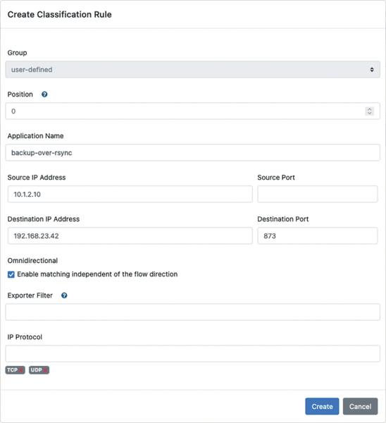 Figure 5: Creating an OpenNMS classification rule.
OpenNMS also lets you import and export classification rules as CSV files, which means you can maintain classification rules in a spreadsheet, for example, or generate them in whatever way you want. One example would be, say, generating rules on the basis of address lists of wallet providers that are freely available on the Internet to detect and prevent crypto mining in the enterprise.
For Grafana, in addition to the OpenNMS Performance data source, you now need another OpenNMS Flow type data source. Finally, the Flow Deep Dive dashboard can be imported from the OpenNMS Helm plugin page. It lets you view the data assigned to this interface by specifying an exporter node and an interface. Because OpenNMS also collects metrics from the interfaces by SNMP, the metrics can be compared directly with the aggregated values of the traffic data, which lets you evaluate how the traffic is composed, besides tracking the utilization of an interface – a great tool for both identifying bottlenecks and prioritizing data traffic on the corporate network.
As Figure 6 shows, throughput is visualized both graphically and as a table for Top N applications, Top N conversations, and Top N hosts, and aggregated by Differentiated Services Code Point (DSCP) values.
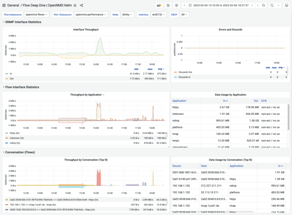 Figure 6: The Deep Dive dashboard is used for flow analysis in Grafana.
In addition to evaluation on this dashboard customized for flow data, RRD graphs for the defined applications can also be generated for each measuring point. You can use the applicationDataCollection parameter to enable this at the adapter level in the telemetryd-configuration.xml file.
If you want to check additional thresholds for this data, you can do so with the applicationThresholding parameter. In this way, alarms can be generated by application. For example, it would be possible to alert on the occurrence of traffic to problematic addresses outside of the corporate network, or to alert on dropping below the target data throughput level during replication between redundant systems.
Scalability
OpenNMS can even collect traffic data in very large environments. The basis for this is the ability to distribute subtasks to minions and sentinels. On the one hand, the querying component acts as a minion, which you can use to query monitored nodes by Internet Control Message Protocol (ICMP), SNMP, or similar. On the other hand, minions also accept logs, SNMP traps, or traffic data (Figure 7).
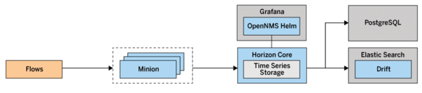 Figure 7: Achieving good scaling through the use of OpenNMS minions as flow collectors.
The metrics and data collected are then passed to an OpenNMS instance or, in larger environments, to sentinels for further processing. In the case of traffic data, this process allows the classifying and enriching flows to be distributed. With this approach, some users have managed to process 450,000 flows/sec, storing more than 100GB/hr of traffic data in their Elasticsearch or Cortex clusters. Figure 8 shows the setup of a larger environment for analyzing traffic data.
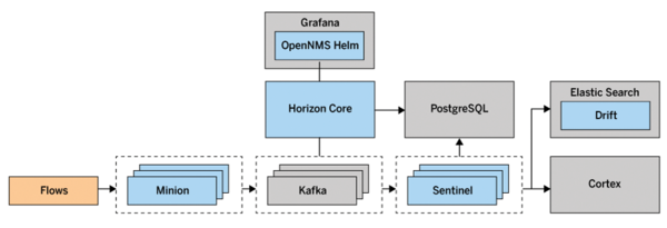 Figure 8: A possible large OpenNMS environment for flow evaluation.
Nephron [8] provides an approach, as well, to aggregating high-resolution flow data over longer periods with an Apache Flink cluster to enable the creation of complex analyses over longer time periods.
Conclusions
Although collecting traffic data with OpenNMS takes some training, it does give you a robust tool for capacity planning and investigating throughput issues or security incidents. The developers have intensively maintained and developed this feature since it was rolled out, always addressing any unusual behavior reported for network devices.
The availability of traffic data in Elasticsearch in a simple but consistent format for all protocols also offers potential for experimentation and for implementing custom use cases for network monitoring.
The OpenNMS Forge Stack-Play GitHub repository [9] contains many container stacks for Docker Compose that demonstrate the interaction of the various components of an OpenNMS Horizon installation. In the minimal-flows/ directory, you will also find an example showing how to process traffic data, which you can try out and use for your experiments.
Infos
- RFC 3917: http://www.rfc-editor.org/rfc/rfc3917.txt
- RFC 3954: http://www.rfc-editor.org/rfc/rfc3954.txt
- RFC 7011: http://www.rfc-editor.org/rfc/rfc7011.txt
- RFC 3176: http://www.rfc-editor.org/rfc/rfc3176.txt
- Helm plugin: https://grafana.com/grafana/plugins/opennms-helm-app/
- Drift plugin: https://github.com/OpenNMS/elasticsearch-drift-plugin
- OpenNMS docs: https://docs.opennms.com/horizon/latest/operation/deep-dive/elasticsearch/introduction.html#ga-elasticsearch-integration-configuration
- OpenNMS Nephron: https://github.com/OpenNMS/nephron
- OpenNMS Forge Stack-Play: https://github.com/opennms-forge/stack-play
« Previous 1 2
Buy this article as PDF
(incl. VAT)
Buy ADMIN Magazine
US / Canada
UK / Australia
Related content
-
DDoS protection in the cloud
 OpenFlow and other software-defined networking controllers can discover and combat DDoS attacks, even from within your own network.
 -
Integrating OCS information into monitoring with OpenNMS
 If you want to manage large IT environments efficiently, you need automation. In this article, we describe how to transfer information automatically from the OCS network inventory system to the OpenNMS network monitoring tool.
 -
OpenFlow and the Floodlight OpenFlow Controller
 Software Defined Networking (SDN) marks a paradigm shift toward a more holistic approach for managing networking hardware. The Floodlight OpenFlow controller offers an easy and inexpensive way to experience the power of SDN.
 -
Floodlight: Welcome to the World of Software-Defined Networking

Software-Defined Networking (SDN) marks a paradigm shift toward a more holistic approach for managing networking hardware. The Floodlight OpenFlow controller offers an easy and inexpensive way to experience the power of SDN.
-
Open Source Security Information and Event Management system
 Systems, network, and security professionals face a big problem managing disparate security data from a variety of sources. OSSIM gives IT security professionals the capacity to cut through the noise and gain wisdom and foresight in defending and managing their networks.
Subscribe to our ADMIN Newsletters
Subscribe to our Linux Newsletters
Find Linux and Open Source Jobs
Most Popular
Support Our Work
ADMIN content is made possible with support from readers like you. Please consider contributing when you've found an article to be beneficial.