« Previous 1 2 3 Next »
Data Analysis with R and Python
On Track
Large volumes of data are most useful if you can study them with intensive data analysis. The open source language, R [1], is a powerful tool for evaluating an existing database. The R language offers a variety of statistical functions, but R can do more.
This article shows how to use R for a sample application that evaluates comet data. An Apache web server visualizes the results of statistical reports – with the help of web technologies such as HTML, JavaScript, jQuery [3], and CSS3, which Python creates in combination with R and the MongoDB [4] database.
Comet Rising
Figure 1 shows how the report generator of the sample application displays the comet data in Firefox. The selection list at the top lets the user select a report variant. If you click on Send, JavaScript sends an HTTP request to the Apache web server, which then generates the report.
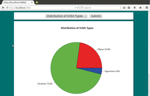 Figure 1: The comet data application in Firefox.
The Python scripts first save the comet data in a MongoDB database. Scripts then parse the data and draw on R to create the report in the form of a graphic, which ends up as a PNG file in a public directory on
...Buy this article as PDF
(incl. VAT)
Buy ADMIN Magazine
Related content
-
A web application with MongoDB and Bottle
 I was recently looking for a stable, flexible, and scalable web application for an ongoing project. It wasn't long until I decided on the NoSQL-based MongoDB.
 -
Introducing the NoSQL MongoDB database
 This overview of the basic concepts, features, and applications of MongoDB emphasizes the advantages offered by this established NoSQL database.
 - Better Crash Recovery with Journaling in MongoDB
- MongoDB 2.4 Released
- MongoDB 6 Features Queryable Encryption
Subscribe to our ADMIN Newsletters
Subscribe to our Linux Newsletters
Find Linux and Open Source Jobs
Most Popular
Support Our Work
ADMIN content is made possible with support from readers like you. Please consider contributing when you've found an article to be beneficial.